1. Introduction

With the recent progress of modalities such as magnetic resonance imaging (MRI) and X-ray computed tomography (CT), vast numbers of high-resolution medical images are being produced at clinical sites. These medical images are playing an important role in the diagnoses of various diseases. The MRI images clearly depict the soft tissues. Therefore, MR images have been an important information source for image diagnosis of the head, abdomen, etc. Brain matter, as assessed by MRI, can generally be categorized as white matter, gray matter, cerebrospinal fluid (CSF), or vasculature. Most brain structures are defined anatomically by the boundaries of these tissue classes. Therefore, a method to segment tissues into these categories constitutes an important step for quantitative morphology of the brain. For example, in brain dock examinations that have been spreading recently, diagnosticians have diagnosed the existence of brain diseases (brain tumor, cerebral hemorrhage, cerebral infarction, etc.) using MR images of several decade slices obtained under different conditions. Because the characteristics of MR images are extremely complicated, diagnosticians in clinical fields cannot sufficiently use the information of MR images, actual cases such as misunderstandings of the meanings of categorized tissues have arisen [1]. Recent surveys of MR brain image segmentation methods [2, 3] have indicated that many difficulties such as in homogeneity and weak boundaries of brain tissues might be associated with the realization of accurate segmentations, despite being important tasks in clinical diagnostic tools. Additionally, it is a difficult and time-consuming task for human experts to combine information from several slices and multiple channels of MR brain images [4]. In fact, MR brain image segmentation persists as a challenging problem because of the complexity of brain structures.

Comparative readings have been conducted to diagnose newly generated lesions and time-dependent changes of known lesions, but results have indicated that a danger exists of overlooking lesions that overlap with the normal structure [5]. After adjusting the registration of images obtained in different days, studies of methods of processing differences of image intensity values have also been conducted. However, false images are generated because of image registration mismatches in details and changes of intensity based on interpolation of image positions [6]. A working group examined variations of diagnostic reading capabilities among doctors in many clinical facilities. That study revealed the existence of great variations in diagnoses using cerebral blood flow single photon emission computed tomography (SPECT). The accuracy of diagnostic reading of MRI is inferior to that of SPECT. Moreover, experiences in diagnostic reading and difficulties for differentiation have been reported as dispersive factors [7]. The few reports of computer-aided diagnosis (CAD) using MR brain images have involved the following: detection methods for the lacunar region using T2-weighted images [8]; automated extraction of brain tissues [9]; extraction boundaries of brain tumors using the three-dimensional region expansion scheme [10]. Most segmentation techniques have relied on multi-spectral characteristics of the MR images, although a few reports of studies have described segmentation from single-channel images. In many clinical applications, it is important to carry out classification of tissues solely from single-channel MR images [11]. By segmenting brain tissues into the significant regions for diagnosis such as the extraction of objective organ and disease region, the development of new application technologies can be expected. However, these are manual processes for most works at present. Even with the recent progress of computer image analysis techniques and MR technology, and despite considerable interest in clinical studies, no automated method for segmentation of brain tissue is available for clinical use.

Normally, segmentation methods for MR brain images are evaluated based on their ability to differentiate between cerebrospinal fluid, white matter, and gray matter in a healthy brain. Otherwise, they are evaluated based on their ability to differentiate between normal tissues and abnormalities. Many segmentation techniques proposed in recent years have been approached with several solutions such as Particle Swarm Optimization [12], genetic algorithms [13], Adaptive Network-based Fuzzy Inference System [14, 15], Region Growing [16], Self-Organizing Maps (SOMs) using Fuzzy C-means [17], SOM-based strategies [18], Growing Hierarchical SOMs [19], and K-nearest Neighbors [20]. Although various approaches have been proposed, each method remains a challenging task in practical use, which entails complex parameter adjustments for determining the category boundaries of brain tissues.

Various methods have been proposed for the segmentation of head MR images [21-24]. Matsui et al. presented a method using Back-Propagating (BP) neural networks based on feature parameters selected by genetic algorithms [21]. Kawahara et al. used the short distance method on feature parameters that were extracted by deforming the texture region [22]. Sato et al. presented a method based on the attributed degrees extracted by fuzzy clustering [23]. In these methods, the operator must specify a representative point for each tissue to be segmented. Consequently, the segmentation result depends strongly on the subjective decisions of the operator. Moreover the methods reported by Matsui et al. are noteworthy: 400 points are used in the segmentation of the brain tissues and other tissues, as are 400 points in the segmentation of white matter (WM) and gray matter (GM). In the method described by Kawahara et al., 30 representative points are used for brain tissue image extraction. These requirements heavily burden operators. Especially for neural network methods, the generalization ability is lowered. Furthermore, the network response is better for training data if the representative points set by the operator are fewer.

However, segmentation without the necessity of specifying representative points is attracting attention. Various methods have been proposed [25-34]. Reddick et al. used SOMs for dividing, and segment tissue by the BP that uses weights of the SOMs for training data [25]. Alirezaie et al. presented a method that combined Learning Vector Quantization (LVQ) with a mapping layer of the SOMs [26]. Sammouda et al. performed segmentation using a Hopfield network, as well as a Bolzmann machine, and analyzed the two segmentation results [27, 28]. In these methods, MR images are taken with various signal parameters: T1-weighted, T2-weighted and proton density weighted images. Then the combination of their brightness values is used as the feature parameter. However, at clinical sites, MR images are rarely taken for the same slice with different signal parameters. Consequently, it is important in clinical applications that the tissues be classified based on a single parameter.

We propose a method for unsupervised segmentation of MR brain images that particularly addresses the self-mapping characteristics of 1-D SOMs [35] and the incremental learning functions of fuzzy Adaptive Resonance Theory (ART) [36]. Additionally, we are developing a diagnostic support system as a CAD system for use with brain dock examinations. For reducing the diagnostician load, this system analyzes the degree of brain atrophy and lesion area quantitatively. We propose an image analysis technique based on nonlinear quantization with 1-D SOMs that can maintain the neighborhood region and integrating categories with Fuzzy ART. This method has the feature of quantifying them based solely on the image characteristics of the diagnostic reading object. Therefore, it is independent of the subjectivity of diagnosticians.

This paper is organized as follows. Section 2 presents a description of our segmentation method used for brain tissue. Section 3 presents a description of the results and discussion of clinical images by analyzing the self-mapping characteristics of the 1-D SOMs. In section 4, we describe construction of the prototype system of CAD for brain dock examinations, and present the field test results of clinical fields. Finally, section 5 presents conclusions.

2. Segmentation Methods for Brain Tissues

2.1. Characteristics of MR Image

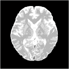
MRI is a technique that produces images of the proton density distribution and relaxation phenomena in biological tissues. Various images are obtainable as follows by varying the signal parameters. A T1-weighted image emphasizes differences in the longitudinal relaxation time of the protons in the tissues. A T2-weighted image emphasizes differences in the transversal relaxation time of the proton in the tissues. The proton density weighted image reflects the proton density.

Among these, the T2-weighted image presents edema and tumors, which have a long transversal relaxation time, with high brightness. Such images are often used most frequently as an enlargement of the CSF region of the MR image [23]. Consequently, this study examines T2-weighted images in which the water content, such as cerebral fluid and pancreatic fluid, is imaged with high brightness, as the target image for tissue segmentation.

Figure 1 shows the type of image regarded as the target of this method. Figure 2 portrays a brightness histogram. The MR image used for this study has resolution of 512 × 512 pixels. The original data have 16-bit brightness level quantization, which is converted to 8-bit (256 levels) images by linear quantization. The first peak in the low brightness range of the histogram corresponds to the background region with low brightness; the second peak is the brain tissue. Although decisive features are few, it is interpreted as presented in Figure 1 as CSF with high brightness.

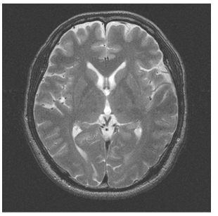Figure 1. T2-weighted image

The brain tissue is divisible into GM, which comprises neurons, and WM, which comprises axons. In T2-weighted images, the GM is located in the high brightness range and the WM is located in the low-brightness range in the brain tissue. The boundary between the GM and the WM is not clearly observable in the histogram. Actually, MRI shows different tissues with similar contrast. Therefore, it is difficult to discriminate tissues with such an obscure boundary from the histogram.

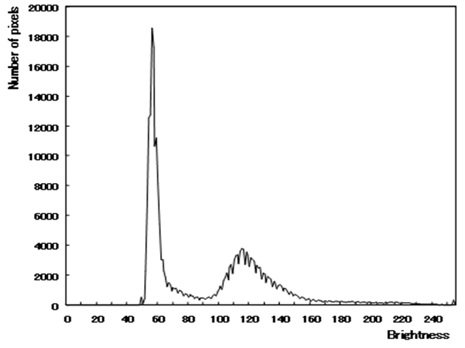Figure 2. Histogram of brightness

2.2. Proposed Method

The determination of tissue boundaries presents a challenging task because the brightness characteristic is not readily apparent on a brightness histogram. Therefore, we hybridize SOMs and Fuzzy ART for the segmentation of brain tissues based solely on the brightness characteristics and distribution of MR images. The proposed method requires no specification of representative points by the operator. It segments brain tissues by self-learning of the image properties, such as the brightness distribution and the edge of brain tissues. This method includes features by which regions with obscure boundaries between tissues can be segmented based on topological mapping the feature parameters exhibited in the MR image.

The proposed method consists of three steps. The first step is to extract the intracranial region from the MR image as a region of interest (ROI). The second step is nonlinear quantization with 1-D SOMs for the intracranial region. The third step is to integrate the number of nonlinear quantization into proper categories with Fuzzy ART.

The detailed procedures are described below.

2.2.1. Extraction of Intracranial Region

Figure 3 shows that we remove the skull and dura mater regions from the original image to extract cerebral parenchyma (GM and WM) and CSF regions for segmentation. For removing these regions, we first transform the gray level image to the binary image using Otsu’s method [37], which comprises the background, skull, dura mater, and intracranial regions. Subsequently, we extract the largest object in the binary image as an intracranial region without skull regions. Nevertheless, dura mater sometimes remains in the intracranial regions because dura mater is distributed between the skull and intracranial regions. It has different distributions depending on the target image.

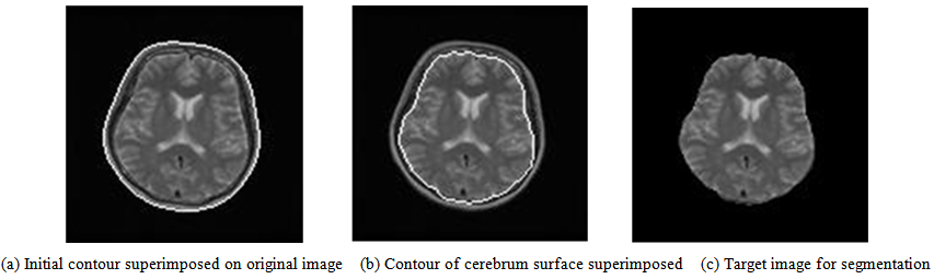Figure 3. Contour extraction process of cerebrum surface

In this study, we use Level Set Methods (LSMs) [38] to extract intracranial regions without dura mater, and use the initial contour of the target image in Figure 3(a). Then the level set functions are initialized according to this initial contour to perform the LSM procedure in Figure 3(b), Figure 3(c) shows that the image of intracranial region for segmentation can be extracted. However, a case exists in which the removal of skull and scalp region is difficult, by the individual difference of the brain structure and the delicate change of the image characteristic. In this case, the brain surface contour can be extracted with only the slightest interaction with diagnosticians, as portrayed in Figure 4. Increase, decrease, and transfer of the nodes forming the brain surface contour can be realized with a simple mouse operation, in Figure 4, these nodes are displayed in the yellow circle.

Figure 4. Window of adjusting the outline to brain surface

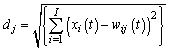
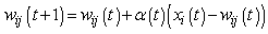
2.2.2. Nonlinear Quantization with 1-D SOMs

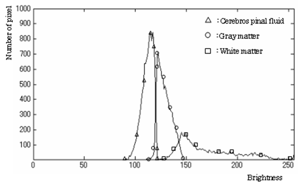
In the T2-weighted image, the boundaries between brain tissues such as CSF and gray, gray and white are not clear because the brightness distribution of each tissue is delicately different and because each tissue forms a peculiar dynamic range in the brightness histogram. That is to say, a subtle distinction exists according to subjects as presented in Figure 5. Therefore, we use the nonlinear self-mapping capability of SOMs to quantize the brightness distribution from topological relations among tissue properties for obtaining proper categories of brain tissues.

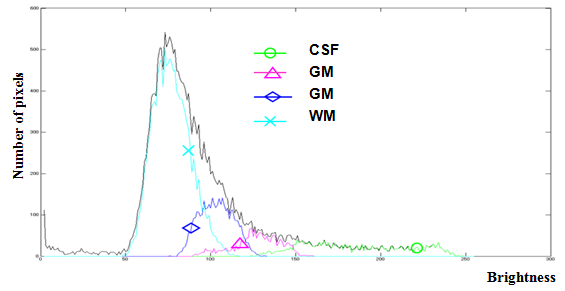Figure 5. Brightness distribution of each brain tissue

The number of created categories depends on the number of mapping layer units with 1-D SOMs. In this study, our segmentation targets are three tissues: CSF, GM, and WM. The segmentation results are not correspondent to these tissues if the mapping layer units are fewer than five units because 1-D SOMs can not maintain the neighborhood region of the own specific characteristics for forming topological relations among these tissues adequately. Otherwise, when the mapping layer units are more numerous than the necessary condition for quantizing a peculiar dynamic range of each tissue, the 1-D SOMs with unnecessary mapping space do not function effectively and cause obscure complexities for reasonable segmentation. While spreading the mapping space of 1-D SOMs, the reasonable quantization of each tissue is conducted based on the brightness distribution of the own peculiar dynamic range. Consequently, based on our preliminary examination, this study adopts a new critical policy that the number of mapping layer units with 1-D SOMs is set to 15, representing the brightness distribution of each tissue. This setting is three times the smallest mapping space that can be maintained in the neighborhood region.

Figure 6 shows that the pixels under consideration are selected randomly from the target image and the local block is defined. As feature parameters of the local block, we calculate the average brightness value of the block, which shows tissue continuity, differences of maximum brightness values, and differences of minimum brightness values that give tissue boundaries. The brightness of the pixel under consideration and the calculated feature parameters are input to the 1-D SOMs to perform self-learning. After learning, the quantization levels are determined based on the weight vector of the pixel under consideration to the average brightness value given as one feature parameter in the local block. The brightness values to be mapped are calculated for all pixels in the target image. For determination of the quantization level of each pixel, the feature parameters used in learning are input again to the 1-D SOMs and the winner unit is determined. Then, the brightness value is assigned based on the quantization level that corresponds to the winner unit labeled in the self-learning process. Figure 7(a) shows a result of nonlinear quantization of the brightness histogram with 1-D SOMs having 15 units of the mapping layer.

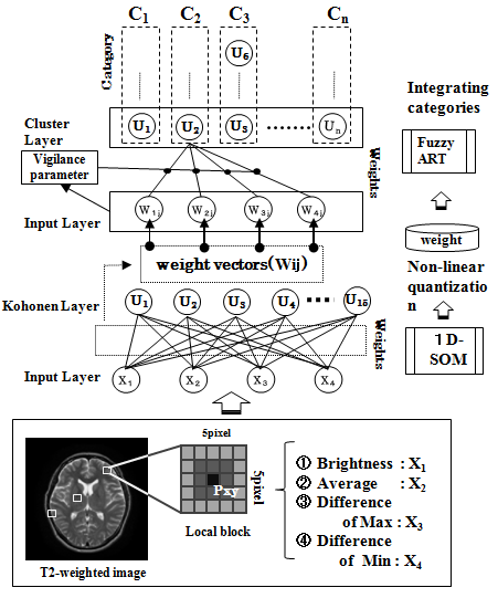Figure 6. Outline of proposed method

The following learning algorithm is used in the SOMs.

1) Let wij (1<= i<= n, 1<= j <=m) be the weights at time t from input layer unit i to mapping layer unit j. The weights are initialized using a random variable.

2) Let xi (1<= i<= n) be the input data at time t to input layer unit i.

3) Calculate the Euclidean distance d_j between x_i and w_ij.

(1)

4) Find the mapping layer unit c which minimizes d_j.

5) Update the weights included in the neighborhood defined by Nc(t):

(2)

where α(t) is the learning coefficient (0< α(t) <1).

6) Repeat steps 2)–5) until the maximum number of learning operations is reached.

In this method, the initial value of α(t) is set as 0.3. The initial value of Nc(t) is set as 3/4 of the number of mapping layer units. It is designed so that both values decrease linearly with time. The learning operations are set empirically as 1,000,000.

2.2.3. Integrating Categories with Fuzzy ART

Fuzzy ART is a theoretical model of incremental learning neural networks that enables the retention of stability and plasticity together [36]. Figure 6 shows that we use the weight vectors of mapping layer units with 1-D SOMs for training data of Fuzzy ART. The quantization levels are defined with the magnitude of these weight vectors. The mapping layer units of 1-D SOMs are arranged according to the learning algorithm of neighborhood region, from a high brightness level to a low brightness level or vice versa. The brightness levels quantized nonlinearly by 1-D SOMs do not accommodate brain tissues such as CSF, GM, and WM, depending on the number of mapping layer units of 1-D SOMs. The main reason is that the brightness distribution of one brain tissue belongs to several quantization levels; particularly those of GM and WM tend to differ according to target images. Figure 7(b) shows the integration results of quantization levels with Fuzzy ART. Using Fuzzy ART after nonlinear quantization with 1-D SOMs, segmentation results corresponding to brain tissues are obtained while maintaining a relation between categories based on approximate brightness.

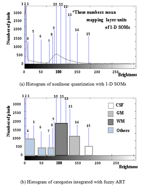Figure 7. Brightness histogram of MR brain image

Brain tissues are classifiable into GM, which comprises neurons, and WM, which comprises axons. In T2-weighted images, the GM is located in the high-brightness range and the WM is located in the low-brightness range in the brain tissue. The mapping labels are based on the relative brightness in T2-weighted images of the brain: among the tissues in T2-weighted images, the CSF is the brightest, followed by GM, then WM. The remaining tissue areas are least bright. The mapping labels are defined in the above order in accordance with the magnitude of the weight vectors. Then Fuzzy ART enables integration of the mapping labels into reasonable brain tissues with a constant scale of the vigilance parameter that controls the classification granularity. Focusing on GM regions of segmentation results, the singular region along the boundary between CSF and WM is observed to be matched with the anatomical brain structures by a diagnostician. Consequently, based on our preliminary examination, we set the vigilance parameter as 0.875.

After learning, the mapping colors are determined based on the weight vector of the pixel under consideration to the average brightness value given as one feature parameter in the local block. The mapping colors are based on the relative brightness value in T2-weighted images of the brain: Among the tissues in T2-weighted images, the CSF is the brightest, followed by the GM, then the WM; all others are least bright. The mapping colors are defined in the above order in accordance with the magnitude of the weight vectors. The map layer units are labeled. The brightness values to be mapped are calculated for all pixels in the target image. In determining the mapping value of each pixel, the feature parameters used in learning are input again to the SOMs. The winner unit is determined. Then, the brightness value is assigned based on the mapping color that corresponds to the winner unit.

3. Results and Discussion

3.1. Results

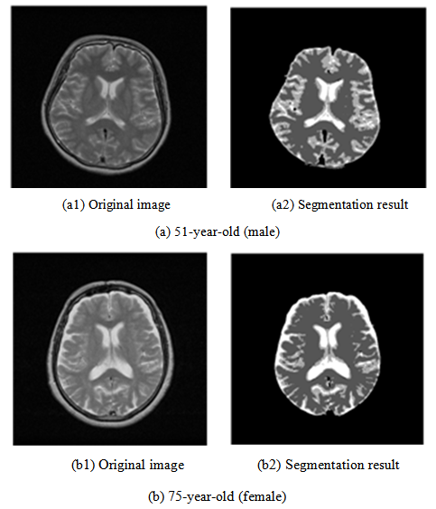
Figure 8 shows segmentation results applied to the proposed method. In observing Figure 8, it is apparent that the CSF is extracted accurately following the high brightness region on the target image. The GM forms a continuous band-shaped region along the boundary between the WM and the CSF. These observations agree with the anatomical knowledge of brain structures. The WM includes small noise components, forming a continuous region. The boundary with the GM is also clear. These results agree with the anatomical knowledge of brain structures. Figure 9 shows a histogram for each tissue in the segmentation result. The histogram corresponds to the brightness histogram presented in Figure 2. It is apparent that the brain tissue, which forms a single distribution in the brightness histogram of the whole image, is classified using the proposed method into WM and GM.

Figure 8. Segmentation result

Figure 9. Histogram of brightness classified by tissue

In addition, the application of the proposed method was tried in clinical image of two examples taken at Akita Kumiai General Hospital. The clinical image presented in Figure 10(a1) represents a case of a patient, a 51-year-old man in whom the there was no indication of brain atrophy according to the diagnosis. Figure 10(a2) shows the segmentation result. In this clinical image, the contrast resolution is generally low, and the boundary between the GM and the WM is especially obscure. Using the proposed method, however, the tissues are classified in accordance with the anatomical knowledge of the structure. The clinical image in Figure 10(b1) represents a case, a 75-year-old woman, who was diagnosed as having progressive cerebral atrophy. Segmentation results presented in Figure 10(b2) show recognizable enlargement of the CSF, especially in the frontal lobe.

Figure 10. Segmentation results of the clinical MR images

3.2. Labeling of Mapping Layer Units

When the target unit fulfilling the requirements is chosen from the mapping results of the SOMs, it is extremely important to analyze the image of weight vectors having a topological relation of each unit in the mapping layer. Regarding utilization of the mapping results, the operator generally carries out meanings for them in many cases. However, the image of weight vectors after learning shows clearly what the mapping layer units have learned on the target image.

Based on the average brightness value given as one feature parameter in the local block, the segmentation carries out labeling of each unit in the mapping layer, based on the brightness properties of brain tissues in the T2-weighted image. Noticing the difference of maximum and the difference of minimum in the local block, both of their values are large, the unit in the mapping layer is defined with the mapping property that works effectively for boundaries between the tissues represented in edges. In other words, analyzing the mapping properties of the SOMs in detail, which are peculiar to the application problem, they can evaluate the validity of the feature parameters, and also specify the effective factors among the feature parameters for the labeling. Furthermore, by including them beforehand with the inputs of the SOMs, the labeling for the mapping layer units can be achieved easily.

3.3. Effective Feature Parameters for Boundaries of Brain Tissues

Many feature parameters are useful for segmentation in MR images. Among these, the brightness of the pixel under consideration is the most informative property. We investigate how the feature parameters (the average brightness value, the difference of maximum, the difference of minimum) affect the clarity of the boundary among tissues with the significant continuity of the brain tissue. To do so, we compare it to the segmentation result in which the distributions of brightness in the local block are used as the input.

Figure 11(a) portrays segmentation results of four feature parameters: the brightness under consideration, the average brightness value, the difference of maximum, and the difference of minimum used as the input. When analyzing the characteristics of each feature parameter based on segmentation results of Figure 11(a), the difference of maximum contributes effectively to detect the boundary from the pixel under consideration to the tissue with higher brightness. Otherwise, the difference of minimum effectively detects the boundary of the tissue with lower brightness. In the T2-weighted image, for example, the GM forms the region surrounded by the CSF and the WM, which has the boundary of the CSF with higher brightness and the boundary of the WM with lower brightness.

When we note the weight vectors of the map layer unit labeled in the GM, both the difference of maximum and the difference of minimum are large and close in comparison with those of other map layer units. Therefore, the map layer unit is characterized strongly as reacting to both boundaries. In addition, for the map layer unit labeled in the CSF, the difference of minimum shows a high value in comparison with the difference of the maximum. The boundaries which the CSF faces the GM and the WM all exist in the lower brightness because the CSF in the T2-weighted image is imaged as regions with the highest brightness.

Regarding the unsupervised learning result of these image properties, the map layer unit labeled in the CSF has the mapping characteristic featured on the difference of minimum, which works effectively for a boundary in the lower brightness.

In segmentation results obtained using the distributions of brightness in the local block, as presented in Figure 11(b), the boundaries between tissues are not clearer than those in Figure 11(a). The mapping characteristic with the continuity of tissue has been emphasized. Especially, particularly addressing the CSF region that shows the degree of the brain atrophy, the boundary faced on the GM is not sharp, and the CSF is segmented as the round region. An expansion tendency on the CSF can be confirmed of the T2-weighted image, in comparison with high brightness region. These show that the distribution of brightness in the local block has the property that inhibits the clarity of the boundaries among these tissues.

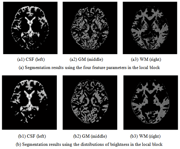Figure 11. Analysis of segmentation results with two input types for SOM

3.4. Adjustment of the Local Block Size

The local block feature parameters are extremely important for segmentation. They depend on the local block size. Consequently, an additional experiment was conducted to study the local block size effect. The local block size is made to change from the first neighborhood of 3×3 pixels to the fifth neighborhood of 11×11 pixels. The segmentation results are presented in Figure 12. In the result based on the first neighborhood, a large amount of noise exists in the WM region. By enlarging the local block to the second neighborhood, the noise components in the WM region are reduced. When the local block is enlarged, the noise components are further reduced, but the region of the GM begins to shrink generally. Furthermore, an incorrect segmentation is produced around the anterior horn of the lateral ventricle, which is misinterpreted as background. The feature parameters in the local block should contain the informative property that can form the region with the brightness characteristic of the original image, which consists of the continuity of tissues and the boundary between tissues. They depend strongly on the local block size. Therefore, local block size optimization is necessary according to the image resolution and the image property of target tissues. Based on these observations, in the case of the image resolution, i.e., 512×512 pixels, the second neighborhood is the most effective. The local block size is set as 5 × 5 pixels for the present study.

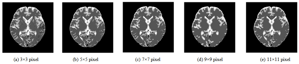Figure 12. Segmentation results according to local block size

3.5. Experiments of Comparison with Conventional Methods

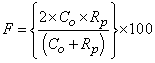
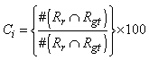
The main contribution of this work is evaluation of the effectiveness of the proposed method, considering the conventional methods that are highly accurate in terms of usefulness as classification techniques. We specifically examine Fuzzy C-means (FCM) [39] and Expectation Maximization Gaussian Mixture (EM-GM) [40] with prior setting of the cluster number, then Mean Shift (MS) [41] without prior setting of the cluster number.

For the experiments, men and women who had undergone brain dock examinations were selected randomly. All were in their 30s to 70s, constituting a total of 10 subjects of MR brain images. To evaluate the classification accuracy of brain tissues, under the supervision of a reading doctor, the operator manually extracted the CSF region that is a metric indicating the progress of the brain atrophy. Then he created ground truth images of 10 subjects. As metrics of the classification accuracy, we applied the degree of coincidence (C_i) and the F value, as calculated from the harmonic mean of degree of reproduction (R_p) and degree of compatibility (C_o) shown in the following equations.

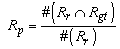(3)

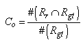(4)

(5)

(6)

Therein, Rr is applied to the extracted region of each method; Rgt was extracted manually as the region of ground truth. In addition, # (R) is the number of pixels in region R.

Figure 13 presents evaluation results of each subject for the classification accuracy using the F value. Figure 14 shows the evaluation results obtained using C_i. In Figure 13, calculating the average value in 10 subjects, the proposed method is 82.9%, EM-GM is 68.9%, FCM is 64.8%, and MS is 47.6%. The proposed method showed the highest value. Furthermore, Figure 14 shows a similar trend: the proposed method was 71.4%, EM-GM was 53.7%, FCM was 49.3%, and MS was 33.7%. These results confirmed the high classification accuracy of our method in all cases. The method is more effective than conventional methods.

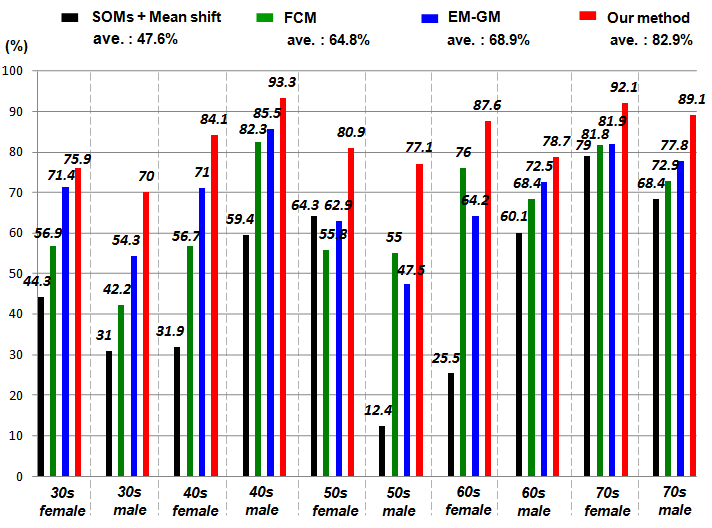Figure 13. Comparison results with degree of F-value

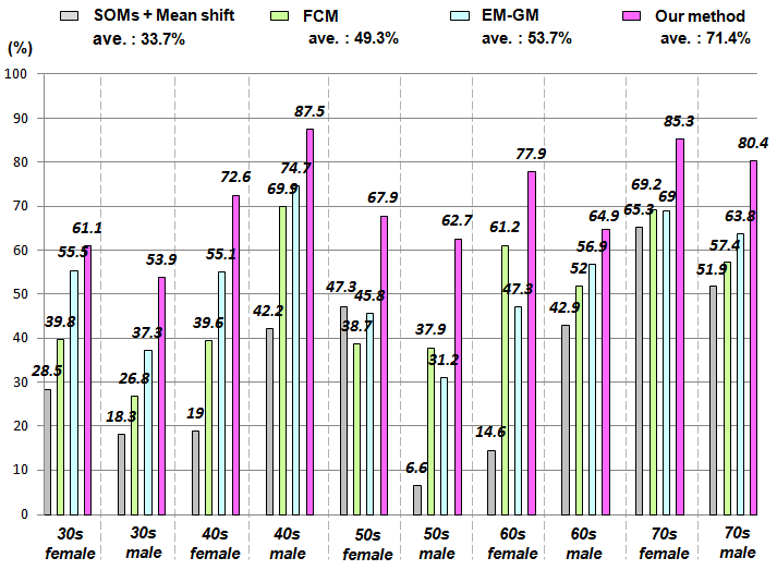Figure 14. Comparison results with degree of coincidence

4. Application to Brain Dock Examinations

4.1. Analysis of Diagnostic Reading Service

Although the human brain atrophies with age [23, 24], reportedly, brain atrophy correlates not only with aging but also with risk factors of cerebrovascular disorders such as drinking and blood pressure [25, 26]. In addition, usual aging alteration must be differentiated from unhealthy brain atrophy because many deformation diseases occurring with brain atrophy such as Alzheimer and Pick illness also exist. That is to say, evaluation of brain atrophy is an important index for use in brain image diagnosis. The cerebral parenchyma mainly comprise WM with GM. The GM consists of neuronal cell bodies; the WM consists of nerve fibers. As a result of the change of the blood vessel circumference structure, the GM volume decreases with aging, but the WM volume does not always decrease with aging [27]. Therefore, it is necessary that GM and WM be classified in addition to CSF, which shows the degree of the atrophy when brain atrophy is evaluated using image analysis. However, it is not easy to evaluate brain atrophy objectively; diagnosticians have been subjectively diagnosing it based on their experience alone.

It is crucially important that the morphological diagnosis of the brain using MRI be carried out using the region of interest and the representative cross section as interactively set to ascertain brain atrophy. This research confronts many problems such as the following. The subject of the operator comes in for the selection of the cross section used as the region of interest and the change in the outside of the setting region can not be detected. In addition, much time is necessary for analyses because handling of the large amounts of data in interactive analysis is not possible. As the most representative tool for automatic analysis of the morphological change of the brain, Statistical Parametric Mapping (SPM) is used [28]. Actually, SPM detects the local morphological change of the brain for research purposes. However, in usual clinical practice, it is difficult for SPM carries out sufficient analyses of brain images with gaps shown. Therefore, an image having thin slice thickness (about 1.5 mm) from three-dimensional imaging modes and interpolation without gaps is necessary for SPM.

Automatic processing by the simple operation only of inputting MR images is extremely important for evaluation of the objective brain atrophy widely in clinical fields such as brain dock examinations. According to differences between imaging parameter and strength of static magnetic field, image quality and signal strength distribution of the MR image greatly change. Therefore, improved efficiency and optimization of the diagnostic reading work must be done, considering variations among imaging devices and clinical facilities, in addition to differences among diagnosticians.

4.2. Construction of a CAD System for Brain Imaging

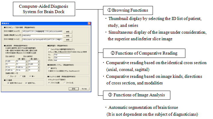
Based on use case analysis of the first diagnostic reading work related to preparation of the diagnostic image report, a prototype of a diagnostic image support system was constructed for use with our proposed method. The composition of a CAD system for brain dock examinations is presented in Figure 15. This CAD system has three characteristic functions: a browsing function that considers the operability of the operator; a comparative reading function that emphasizes the relevance to images in the diagnostic reading work; and an image analysis function which maps only the image characteristics of the diagnostic reading object. This CAD system produces medical images with header information that conforms to the Digital Image and Communication in Medicine (DICOM) 3.0 standard for objects. It makes all folders and files existing under working directory as browsing objects.

Figure 15. System structure

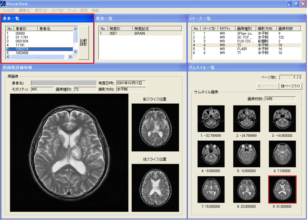
4.2.1. Browsing Function

The top window of browsing is presented in Figure 16. The analysis of all header information related to the DICOM files (MR brain images) has finished on displaying window of Figure 16. The upper part of the browsing window is composed in order of the left side in each window of the patient list, study list, and series list. The right side of the lower browsing window is the thumbnail display region. The left side of the lower window is the region displaying the original image chosen in the thumbnail display region. In addition, it is possible to display anterior and posterior slice images of the original image. On the patient list window, the squeezing of patient information as an object is simply possible by choosing age and sex from the menu by adjusting the medical care purpose. The procedure of diagnostic reading is executed by choosing the patient ID first, and choosing the study ID next in the order which searches the series list of an object. In addition, the thumbnail images of slice positions are arranged as acquired by choosing a corresponding series ID from the series list. The example of Figure 16 is that of a case in which the axial image of T2-weighted image was chosen.

Figure 16. Browsing window

The original image is expanded and displayed when the slice image of the attention is chosen from the thumbnail display region. Simultaneously, anterior and posterior slice images are displayed. Change of the slice position can be realized in the simple operation of clicking the anterior or posterior slice, whereas the expanded original image is observed carefully.

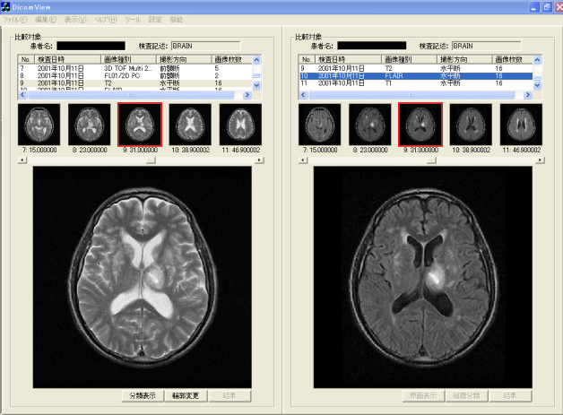
4.2.2. Comparative Reading Function

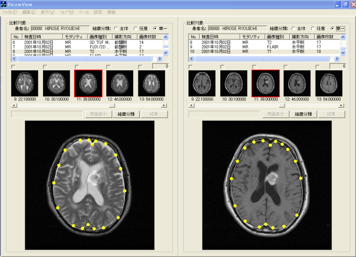
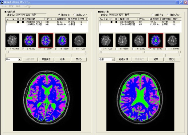
Comparative reading is undertaken to choose a "comparative reading" menu button of the browsing window. The condition is switched to comparative reading window in the identical slice cross section (axial, coronal, sagittal) presented in Figure 17. The left side in the window presented in Figure 17 is a T2-weighted image. The right side is the FLAIR image, in addition, both images are the same slice position in identical axes. When the object of comparative reading is switched, comparative reading which optionally changed image types, slice directions, modality, etc. is possible by choosing corresponding series ID from the series list, which are displayed respectively in the upper part in the left window and right window. The change of the slice position is executed merely by clicking thumbnail images displayed under the series list. In addition, slice positions in right and left change: they are linked. Therefore, diagnosticians are expected not to undergo stress for useless operations such as ordering and rearranging images. Consequently, they can concentrate on their original diagnostic reading work.

Figure 17. Window of comparative diagnostic reading

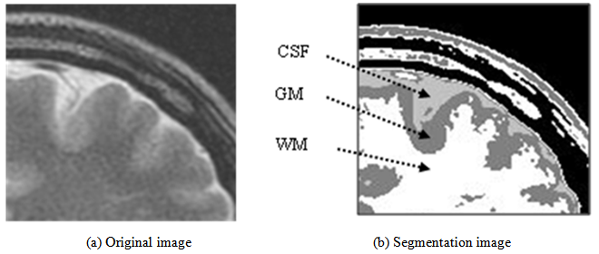
4.2.3. Comparative Reading Function

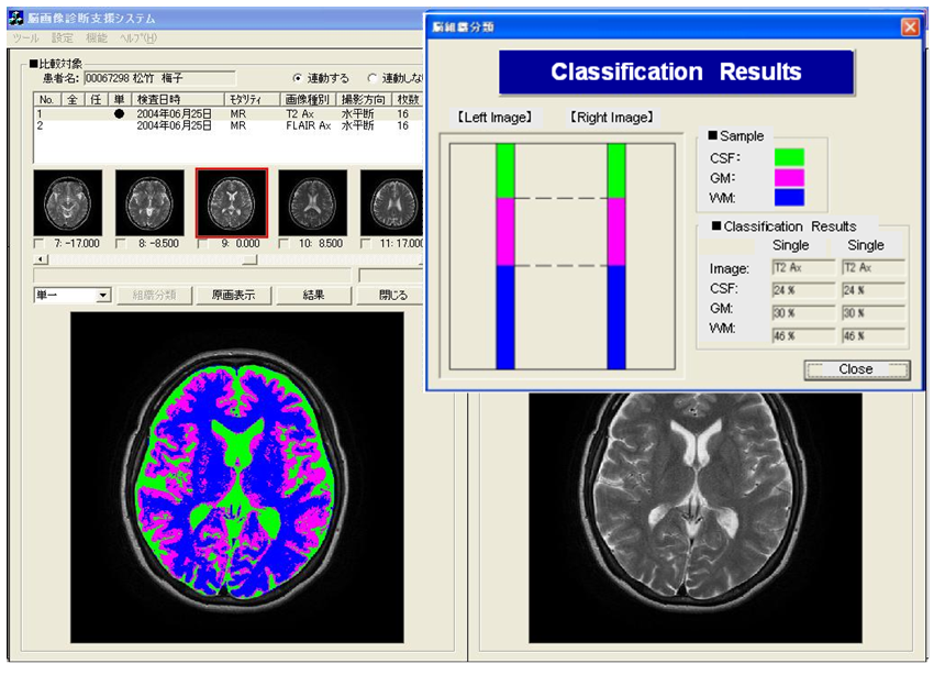
This image analysis function has features by which the brain tissue of the diagnostic reading object can be classified automatically, merely by learning image characteristics such as edge and brightness distributions. No intervention of diagnosticians is necessary. In the application of this image analysis function, extraction of the lesion area in comparative reading and quantification of the brain atrophy with aging can be realized because segmentation of the region in which the boundary of brain tissues is unclear becomes possible. In the example of T2-weighted image presented in Figure 18, the boundary of CSF imaged as a high brightness region and GM, and the boundary of WM and GM, although these boundaries are indistinct to confirm on original image in the visual observation, the boundaries between tissues can be confirmed clearly in the segmented image.

Figure 18. Segmentation of brain tissue

Diagnostic reading of the analytical result can be executed using the comparative reading function. Figure 19 presents an example portraying the original image at the left side and the segmentation result of the brain tissue at the right side in the window. Diagnostic reading is possible, whereas the validity of the segmentation result is contrasted with the original image. By clicking the graphical representation button, it is possible to obtain the occupation proportion (%) of each tissue in making the intracranial region be 100. Simultaneously, diagnostic reading for multiple slice images is realized by putting a check in the thumbnail image displayed under the series list, as it is presented in Figure 20, by totaling the segmentation result of chosen each slice image, and by graphing the result. Therefore, a general tendency and partial tendency in an axial section of interest can be grasped by showing it in comparison to the segmentation result of 1 slice image of them at the right side. Still, these segmentation results can be output as a CSV-type style file.

Figure 19. Case A of diagnostic reading using our proposed method

Figure 20. Case B of diagnostic reading using our proposed method

4.3. Field Test

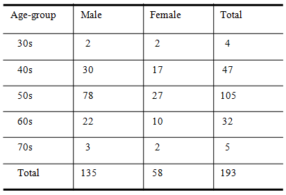
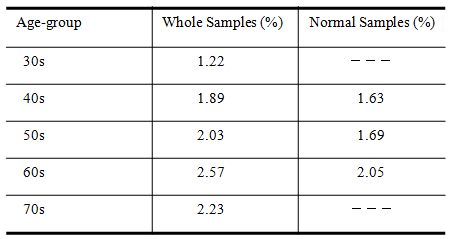
For medical examinees of brain dock examinations at Akita Kumiai General Hospital, field tests were conducted of the effectiveness of this CAD system in the diagnostic reading work. MR images as a diagnostic reading object are the T2-weighted image and the FLAIR image taken in MRI modality (EXCELART1.5T; Toshiba Medical Systems Corp.). These are all axial images of slice gaps of 6 mm. The T2-weighted image emphasizes the difference in the transversal relaxation time between protons in the bio-tissues. It is used most frequently in the clinical field because it can present edema and tumors with high brightness despite their long transversal relaxation time. The MR image resolution is 512 × 512 pixels, and the brightness level is 16 bit.

The evaluation objects are MR images (6324 images) of 193 patients (135 male, 58 female), who had medical examinations during brain dock examinations at Akita Kumiai General Hospital from January 2004 through November 2005. These image datasets were acquired in all identical imaging parameters. No change of the signal strength occurred by the difference of the parameters. For the 193 examples, the breakdowns of age and sex are presented in Table 1. For all medical examinees of brain dock examinations, 193 examples, and the patient group who were diagnosed with the normal-range, we quantified the atrophy with age independence for 34 patients (23 male, 11 female). The results for all medical examinees are presented in Figure 21. The result of a patient group of people diagnosed with the normal-range is presented in Figure 22. The height lines on each sample point show the standard deviation as a degree of dispersion. Table 2 presents results in which they are arranged.

Table 1. Details of age-group and sex of people with brain dock

Table 2. Details of standard variation with age-group

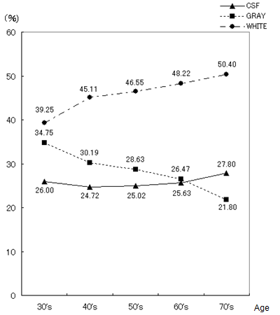Figure 21. Aging tendency of brain atrophy overall

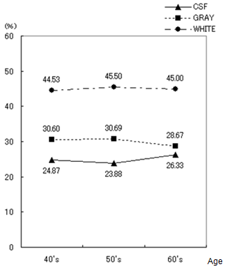Figure 22. Aging tendency of brain atrophy vs. normal

As shown in Figure 21, the proportion generally increases with age, when a degree of atrophy is noticed from the space of CSF. Especially, the tendency is pronounced for patients in their 70s. For patients in their 40s and 50s, the value of the standard deviation showing a variation of individual specificity is small, but in patients in their 60s and 70s, the values are large. Although the middle age layer (patients in their 30s, 40s, and 50s) shows only slight progress of the atrophy comparatively, individual specificity is not recognized, but there is clearly individual specificity in progress of the atrophy with the aging (patients in their 60s and 70s). No clear reference is possible because a difference exists in the sample numbers of each group. Especially, patients in their 70s are few: only five. However, it can be estimated that atrophy appears remarkably with aging. By recommending and carrying out strict medical examination of brain dock examinations in patients beyond their 60s, when the progress of atrophy is remarkable, it can be expected that general atrophy occurring with aging can be found to be related to individual specificity. Comparative readings for the image set of the time series of each medical examinee is possible.

However, comparison of Figure 22 with Figure 21 shows that the value of the standard deviation in each generation is small, and the proportion of CSF in the middle age layer (patients in their 30s, 40s, and 50s) has been stabilized at a low value. In addition, when the breakdowns of patient group who were diagnosed with the normal range are analyzed, numbers of samples of the middle age layer can be ensured: patients in their 30s present 1 example, patients in their 40s present 15 examples and patients in their 50s present 16 examples. In contrast, the number of samples decreases sharply with the progress of aging: patients in their 60s present 3 examples and patients in their 70s present 0 examples. As one reason, cases diagnosed as asymptomatic cerebral infarction (lacunar infarcts) increase with age.

In the aging society, most medical examinees have lifestyle-related illnesses as a background. Especially, preventive measures against cerebrovascular disorders become important, when hypertension, hyperlipidemias, diabetes, and cardiac diseases are diagnosed. Stimulating improvement of healthy lifestyles to prevent asymptomatic cerebral infarction (lacunar infarcts) can forestall or prevent symptomatic cerebral infarction. Consequently, as presented in Figure 21, quantitative detection of atrophy with aging is an important purpose for diagnostic imaging.

Next, representative original images and the segmentation results in each generation are presented in Figure 22. The CSF is extracted appropriately along the high brightness region on the original image. The GM (GRAY) forms the banded region along the boundary between the WM (WHITE) and the CSF. These segmentation results agree with the anatomical structures of the brain. Furthermore, segmentation results agree with the anatomical knowledge that the brain atrophy concurs with the extension of third ventricle and lateral ventricle. From the viewpoint of a diagnostician evaluating the validity of the segmentation results, the following opinions were issued. Diagnostic reading in comparison the segmentation result of each tissue with the original image directly, and the mechanism which can link observing slice position in left window and right window, when they are necessary, these functions are very effectively interesting.

The facts described above show that the burden to diagnosticians in the clinical field can be reduced. The effectiveness of this CAD system of brain atrophy in diagnostic image process was confirmed. In brain dock examinations, reproducibility of image diagnosis is obtained irrespective of the clinical facilities or imaging model. However, the present evaluation is merely that of results of MR images from an imaging model used at a specialized facility. In our future work, similar evaluation experiments must be conducted for other JA group facilities in Akita Prefecture. Moreover, it is necessary to clarify the actual conditions of variation among MRI devices and clinical facilities.

5. Conclusions

As described in this paper, we proposed an unsupervised segmentation method that hybridized 1-D SOMs and Fuzzy ART based solely on the brightness distribution and characteristics of MR brain images, without requiring specifications of representative points by the operator. Additionally, we have constructed the CAD system for brain dock examinations, estimating the degree of brain atrophy according to age. Based on viewpoints of the segmentation method for the brain tissues in MR head images, we analyzed characteristics of self-mapping in the 1-D SOMs with a narrow mapping space. The average brightness value, the difference of the maximum, and the difference of the minimum in the local block with the pixel under consideration as the center were effective as feature parameters to be input to the SOMs. Evaluation experiments showed that the tissues are classifiable. The continuity and boundaries of the brain tissues can be clarified, suggesting segmentation that agrees with the anatomical knowledge of brain structure. For diagnosticians who evaluate the validity of segmentation results, these segmentation results agree with the anatomical structures of the brain. Nonlinear quantization with 1-D SOMs and integrating categories with Fuzz ART produced reasonable segmentation results matching the judgments of brain-atrophy diagnosticians.

The CAD system for brain dock examinations based on youth case analysis of the diagnostic reading work was proposed forderating of medical specialists in quantitative analysis of the degree of brain atrophy, and the prototype system was developed. The browsing function and comparative reading function of this CAD system offer the prospect that diagnostic reading work in the clinical field can be supported. Results of a field test of 193 examples of brain dock examination data from Akita Kumiai General Hospital showed the progress brain atrophy with aging. The following points were clarified.

(1) Generally the proportion of CSF showing the degree of the atrophy with the aging increased. Especially in patients in their 70s, the tendency was remarkable.

(2) For patients in their 40s and 50s, the standard deviation showing the variation of individual specificity was small, but the value was large for patients in their 60s and 70s.

Although no great differences were found among individuals in terms of specificity, the middle age layer (patients in their 30s, 40s, and 50s) showed slight progress of atrophy, but clear individual specificity was apparent with aging (patients in their 60s and 70s). Image analysis functionality must be improved to enable the automatic detection of asymptomatic cerebral infarction (lacunar infarcts) diagnosed mainly from brain dock examinations. Field tests will be conducted continually.

ACKNOWLEDGEMENTS

This study was conducted as a part of the Collaboration of Regional Entities for the Advancement of Technological Excellence from Japan Science and Technology Agency (JST) and the Ministry of Education, Culture, Sports, Science and Technology of Japan.