Evans Annan B.1, Abraham Aidoo B.2, Chukwugozie Ejeh J.1, Asamoah Emmanuel1, Daniel Ocran3
1Department of Oil and Gas Engineering, All Nations University College, Koforidua, Ghana
2Department of Geoinformatics, Ghana Water Company Limited, Accra, Ghana
3Department of Petroleum Engineering, University of Mines and Technology, Tarkwa, Ghana
Correspondence to: Evans Annan B., Department of Oil and Gas Engineering, All Nations University College, Koforidua, Ghana.
| Email: |  |
Copyright © 2019 The Author(s). Published by Scientific & Academic Publishing.
This work is licensed under the Creative Commons Attribution International License (CC BY).
http://creativecommons.org/licenses/by/4.0/

Abstract
Geostatistical methods have been applied to a reservoir in Jubilee oilfield, south-western Ghana, to analyses the distribution patterns of porosity, permeability and thickness. The spatial characteristics of porosity, permeability and thickness in this study were described through geostatistical analysis. The methods implemented include simple kriging (SK), ordinary kriging (OK), sequential indicator simulation (SIS) and sequential gaussian simulation (SGS). Experimental variograms and corresponding anisotropic variogram models were fitted to distribute flow unit data for porosity, permeability and thickness in the reservoir at well locations. The nugget effect, range and sill were used as key input parameters for variogram computation and modeling. Descriptive statistical analysis is performed to provide the means for geostatistical modeling. The statistical analysis yielded coefficient of variation values of 0.4042, 0.5217 and 0.3721, indicating better prediction for the porosity, permeability and thickness. 3D spatial-based maps for porosity, permeability and thickness were generated and analysed critically with respect to their significant variations in the reservoir. Analysis of the results from the spatial-based maps showed that porosity, permeability and thickness were distributed uniformly at the center towards north-east direction of the reservoir. It is also observed that both kriging methods gave good estimate. However, gaussian simulation provided more details to quantify the reservoir heterogeneity than kriging methods. The porosity, permeability and thickness estimated from SK method ranged between 17.01 to 22.54%, 158.48 to 2089.29 mD and 10.04 to 29.32 ft while OK method fell between 17.10 to 22.34%, 1023.29 to 3019.95 mD and 9.85 to 29.01 ft. Finally, regression analysis is performed for generated models. Quantile normalization plots were constructed to establish relationship between the simulated (SGS) data and estimated (kriging) data via real data for validation. The major contribution of this study is that, geostatistical reservoir modeling has been used to analyse the spatial behaviour of porosity, permeability and thickness for performance prediction of Jubilee oilfield.
Keywords:
Kriging, Gaussian Simulation, Geostatistics, Thickness, Porosity, Permeability
Cite this paper: Evans Annan B., Abraham Aidoo B., Chukwugozie Ejeh J., Asamoah Emmanuel, Daniel Ocran, Mapping of Porosity, Permeability and Thickness Distribution: Application of Geostatistical Modeling for the Jubilee Oilfield in Ghana, Geosciences, Vol. 9 No. 2, 2019, pp. 27-49. doi: 10.5923/j.geo.20190902.01.
1. Introduction
The production of map of variable parameter from limited sample data has been a prevailing problem in the oil and gas industry for years. In order to address this problem, geostatistical methods are commonly used in creating a map to capture uncertainties associated with the use of limited sample data in property estimation. It is also a suitable method for effectively analyzing the petrophysical properties data and mapping of subsurface property values at unsampled points (Johnston et al., 2003). Since late twentieth century, geostatistical techniques have been universally recognized for characterization of petroleum reservoirs. The technique was introduced in reservoir characterization purposely for the development of heterogeneous reservoir and the fact that oil industry is capital intensive; companies were compelled to use innovation and cheaper means to optimize hydrocarbon recovery Deutsch et al., 1996). However, unlike deterministic methods, geostatistical methods were introduced in the oil and gas sector to predict and model the reservoir with precision. Geostatistics provides numerous reliable results (Zhao et al., 2014; Zarei et al., 2011). The application of geostatistical methods in oil fields may result in the production of an average image or a set of equally probable images describing the spatial distribution of petrophysical variables, emphasizing the various rock types, porosity, permeability and fluid saturation. Each of the equiprobable images comprises of a two or three-dimensional grid model containing millions of nodes that represent the internal structure of the field including petrophysical parameters and morphology (Deutsch and Journel, 1992; Srivastava, 2004). Over the years, the use of geostatistical conditional simulation for reservoir property prediction is on the wide spread. Geostatistics generates models or realizations of spatial distribution of categorical variables such as geological units and lithotypes including numerical variables like porosity, water saturation and permeability. The outputs from stochastic simulation produce equiprobable image descriptions that have the same probability of occurrence. Demonstrated from several case studies, the models (image descriptions) are based on probabilistic approach that has been proven to be the most appropriate method to quantify spatial heterogeneity in oilfields. Stochastic models (image descriptions) allow detailed modeling of intrinsic complexities to produce equally probable scenarios to describe the internal architecture of reservoirs at inter-well locations and low conditioned regions. The models are usually created from small dataset extracted from experimental data mainly to describe spatial distributions of relevant petrophysical properties of oil fields (Matheron et al., 1987; Journel and Alabert, 1988; Journel and Hernandez, 1989; Perez and Journel 1990; Goovaerts, 1997). Geostatistics improve predictions by providing reliable numerical models. The core mandate is to construct a more robust and realistic model of the reservoir spatial heterogeneity using techniques that do not average relevant reservoir properties. Like conventional deterministic method, it captures known unquestionable “hard” data and informative “soft” data (Wilson et al., 2011).The Stanford Geostatistical Modeling Software (SGEMS) is an open-source computer tools for solving spatially-related problems. It provides geostatisticians with a user-friendly environment and wide selection of algorithms to construct 3D numerical model (Kelsall and Wakefield 2002). The application of SGEMS facilitates detailed understanding of geostatistical estimation and conditional simulation algorithms for enhanced 3D visualization (Kelkar and Perez 2002; Remy et al., 2004; Geoff, 2007; Remy et al., 2009). However, the creation of spatial-based maps is very crucial to depict the characteristics of the real spatial attributes of an oilfield. In this regards, geostatistical conditional simulations are widely-used methods which can quantify the unknowns in a reservoir description to describe spatial attributes of reservoir properties. Mapping the distribution pattern of reservoir properties using geostatistical methods can consequently help in proposing optimal recovery processes and, to improve reservoir performance prediction. In the proceeding chapters of this research, SGEMS is used to evaluate the distribution of porosity, permeability and thickness in an oilfield. In addition, reservoir property estimation is performed in building three-dimensional spatial-based maps (static models) of the reservoir properties; and the models were used to perform comparative analysis of geostatistical techniques.
2. Field Description
The Jubilee Oilfield is located in the Gulf of Guinea near the Ghana and Côte d’Ivoire border along the coast of the western region of Ghana, 60 km deep offshore. Discovery of the field was initiated in June 2007, with average water depth of 1250 meters. It forms part of the South-Atlantic Ocean and lie between deepwater Tano and West Cape Three point blocks in Ghana. The various blocks within the field are under the ownership of the Ghana National Petroleum Corporation (GNPC) and National Petroleum Authority (NPA). Tullow oil developed the Jubilee offshore oil field after the discovery by Kosmos Energy. Production of oil from the Jubilee field started in 2010. It recorded average production rate of 150,000 barrels per day and total proven reserves was around 3 billion barrels. The amount of gas in the field is estimated to be 1.2 trillion cubic feet, representing 162 million barrels of oil equivalent. The participated oil companies discovered a total of more than 15 wells in the western territory (Abrokwah, 2010; Kastning, 2012). Figure 1 shows the map of the study area.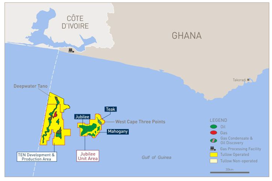 | Figure 1. Map of Ghana’s hydrocarbon discoveries showing location of the Jubilee Oilfield (Tullow, 2013) |
2.1. Geological Setting of Study Area
The field is largely characterized by a continuous stratigraphic trap combined with thick hydrocarbon belts of about 600 meters. The reservoir is found in the deep offshore Tano basin within Gulf of Guinea hydrocarbon depositional belt and extends to the Ghana-Ivory Coast basin. The field consists mainly of cretaceous rocks, specifically sandstones as the main lithology. The field forms part of the Turonian and Santonian formations and consist mainly of cretaceous rocks which are bounded in the west by the St. Paul fracture zone. The basin originated as a result of the tensional movement of the Atlantic Ocean separating Africa and the South America. This resulted in the deposition of rich thick organic shale in the Turonian and Cenomanian era. The environment of deposition is made up of thick clastic sequence and turbiditic fan channeled into the basin from several rivers. The Turonian-Cenomanian shale and Albian sandstone constitutes the major source rocks of the Tano Basin. The reservoir rocks evolved from the sloped Albian sandstone and turbiditic faulted-fan sandstones of the Turonian. Trapping of hydrocarbons are largely influenced by stratigraphic and structural features (Brownfield and Charpentier, 2006). Initial rift from sedimentary infill of the western Basin consists of Lower Cretaceous sandstone ranging from Aptian to Lower Albian. The lower section is of marine origin with thickness more than 4000 meters. The marine influence increases in the upper sections from which oil and gas reservoir are deposited within thick sandstone units. A large tilted block which forms the Central Tano structure is surrounded by Kobnaswaso formation and thick rift-units of the Devonian rocks (Cretaceous or Paleozoic). In the offshore zones, the Kobnaswaso formation is characterized by thinly interbbed lithic and feldspathic shale and sandstones. The sandstones are angular and round in shape and are generally fine-grained to conglomeratic poorly sorted. Thick sequence of shale and sandstones of the formation including other lithologies has been partially penetrated by the deep offshore wells of which nine of them constitute the offshore Western Basin wells (GNPC, 1989). Figure 2 shows the location map of wells in the study area.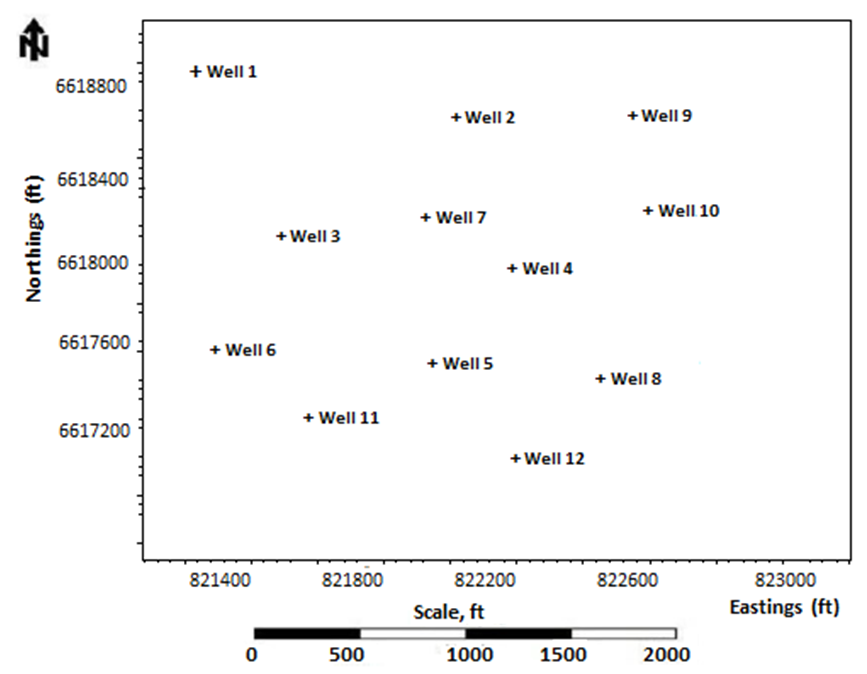 | Figure 2. Location map of wells in the study area |
3. Methodology
This study presents geostatistical numerical simulation approach for the characterization of an oilfield. For this research, reservoir flow unit data for porosity, permeability and thickness obtained from 12 actively producing wells in the offshore Jubilee oilfield were used to perform geostatistical analysis. The data covers about 350 points taken from each well in a reservoir in the Jubilee oil field. The flow unit data was taken from cores to logs for description of several geological cross sections throughout the field, including top, thickness, porosity, permeability (in log form) at different well locations. The methods adopted included: estimation of petrophysical variables at unknown locations conditioned to kriging algorithms and simulation of variables (porosity, permeability and thickness) for generating multiple equiprobable property images describing the reservoir heterogeneity. Conditional simulation (i.e., sequential gaussian simulation, sequential indicator simulation) and kriging algorithm were implemented for the property modeling stage of this research using the gaussian simulator (SGEMS). 3D grid model of the reservoir was constructed with a cell size of 80 x 80 x 20. Total cells of 128000 with seed value of 14071789 were obtained for the grid model. The porosity, permeability and thickness data were scaled up and distributed realistically in a three-dimensional grid by assigning a value for each property estimated. Variogram models were computed for these properties. Spatial-based maps were generated for porosity, permeability and thickness to evaluate their variability in the reservoir. The different reservoir model descriptions (image maps) obtained from the conditional simulation runs were discussed and analysed. Finally, regression-based analysis is performed to validate the reliability of the generated models. Figure 3 shows the flowchart of methodology used.
3.1. Application of Geostatistical Modeling Methods
Gaussian simulation is a conditional geostatistical method that utilizes the kriging mean and variance to produce a gaussian field. Gaussian random field makes use of gaussian probability density functions. It also uses simulation function parameters and input data. The sequential gaussian simulation (SGS) technique is mostly used in modern times because it is reasonably effective, simple and flexible (Pyrcz et al., 2014). In SGS algorithm, the variance and mean of the distribution function at a given location specified in the simulation path is predicted by kriging approach and kriging variance. The value obtained from the distribution is commonly used as conditional data. More often, the log transform of the actual data into gaussian distribution may be needed by the normal score transform (Remy et al., 2009).
3.2. Kriging Algorithm
The mining industry in the early twentieth century 1950s realized that classical statistics were inappropriate for prediction of ore reserves. For this reason, D.G. Krige, a South African mining engineer in collaboration with H.S. Sichel, a statistician proposed a new of predicting properties at unsampled location. George Matheron further researched into Krige’s ideas and formulated the concept into a single framework. Matheron discovered the word Kriging to acknowledge the work of Krige. In this perspective, kriging was initially designed for reserve estimation until it spread to areas of earth science. Geostatistical methods gained wide acceptance in the petroleum industry in the mid-to-late 1980s and were accepted gradually (Krige, 1951; Lake et al., 2007). However, attempting to be unbiased consequently ended in overestimation of values and underestimation of high values. At that time, Daniel Krige and Georges Matheron proved to be critical (Pyrcz et al., 2014). Kriging and cokriging geostatistical methods are commonly used for interpolation. Both techniques are forms of univariate and multivariate linear regression-based models for estimating point over a given region. The strength of kriging as an interpolation technique depends largely on its ability to describe anisotropy of geological variables using spatial covariance model, producing map that depict more geological features (Lake et al., 2007). The variables and their associated weights at given location are related by the equations (1) and (2), shown below.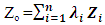 | (1) |
whereZo = value at the un-sampled location to be estimated λi = weight of the regionalized variable Zi = the regionalized variable at a given location di = the distance between the un-sampled and sample locationp = given power 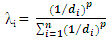 | (2) |
3.3. Simple Kriging
As a rule-based assumption for simple kriging (SK), a value at an unsampled point can be estimated trivially. For SK estimations, the global mean is usually held constant over the entire region of estimation (Kelkar et al., 2002). SK uses the Equation (3) in property estimation: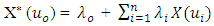 | (3) |
where = the value to be estimated
  = a nearby sample value at location
 = the total number of samples selected within a search neighborhoodλi = the weight assigned to each sampleλo = a constant parameter
3.4. Ordinary Kriging
Ordinary kriging (OK) is a geostatistical technique which estimates variables locally using interpolation. Krige and Matheron proposed this linear interpolation method with the purpose of minimizing the volume of variance effect. They suggested on a linear method because it provided the least discrepancies (differences) between actual and estimated mine grades. In OK, the regionalized variables are assumed to be stationary where the mean (m) remains unknown. When using OK, all the data points with no sample value are assigned a significant value using a weighted linear combination of the known sample variables (Mpanza, 2015).
3.5. Variogram Computation and Modeling
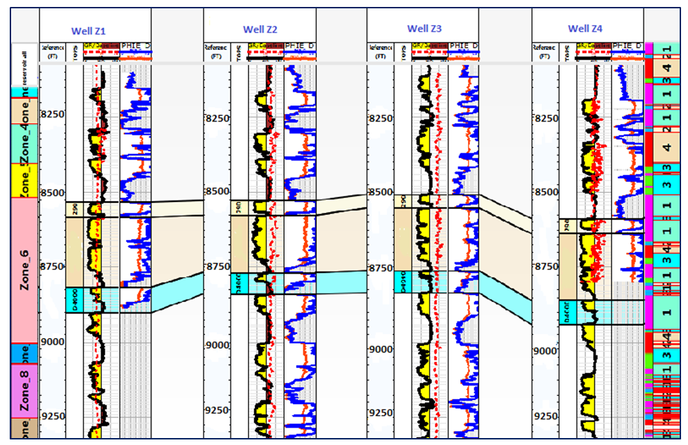
Clark (2001) defined a variogram model as a graph describing the expected difference in value between pairs of samples relative to their orientation and distance apart. Journel and Huijbregts (1978) also defined variogram as a function that captures the variability of samples based on expectation of the random field. The different types of variogram models introduced are spherical, gaussian, exponential, linear and power model. The selection of a model depends on the arrangement of the data points. How the data points are arranged will suggest the variogram model that best fit the variable to be modeled. The reason behind the choice of variogram model is the shape suitability to match the observations (Clark, 2000). Basically, variogram is the measure of dissimilarity or increasing variance between pair of points as a function of lag distance. Information from the variogram is used to seek ideas about grades in an ore deposit based on weighting the surrounding samples. The variogram shows the difference in sample values as the distance increases in a given direction (Mpanza, 2015). Variogram is computed from equation (4) as shown below: 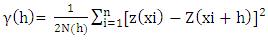 | (4) |
whereh = separation distance = variogram or semi-variogramZ(xi) = value of sample at location xiN(h) = total number of sample pair for lad distance hZ(xi+h) = value of sample located at point xiThe higher the variogram value the more dissimilar of the value of the attributes being examined.
4. Results and Discussion
4.1. Petrophysical Analysis
In this research, a detailed petrophysical analysis is performed on the reservoir within the zone of interest where the studied wells are located. The zone under consideration is between 8250 ft and 9250 ft as shown in Figure 4. The log analysis revealed two distinct zones for the reservoir. The top zone (upper portion) of the reservoir comprised of thick clean sands as indicated by the signature of the gamma logs. The most productive top zones of the reservoir are from 8259 ft to 8526 ft. The top section for the reservoir zone has thickness of 16.5 ft with average high porosity value of 25.1%, respectively. The analysis also revealed net to gross ratio of 97.57% and net pay thickness of 16.1 ft. It is important to note that the reservoir consist of a vast total rock volume characterized by thick sand sequence with few non-reservoir features. Moreover, a very low significant water saturation of 8% was obtained for the top zone, which compliments high hydrocarbon saturation value of 92%. The base portion of the reservoir is characterized by less clean sands interbedded with muddy shale sediments as shown by the gamma ray log. This suggests the presence of fairway sand bodies deposited in fan system within the part of the reservoir under consideration. The reservoir recorded lower porosity readings of 17.0% in the lower sections, which may be an indication of high shale volume. The computed volume of shale in the reservoir zone is slightly high which could portray a tight reservoir rock formation with low sand sequence. The logs indicated in Figure 4 showed good petrophysical features. It revealed high concentration of reservoir quality sands trending from northeast to the southwest sections. This could prove to be a prospective zone for future drilling projects. Figures 4 and 5 show the petrophysical logs and correlated wells for the reservoir in the sector of study.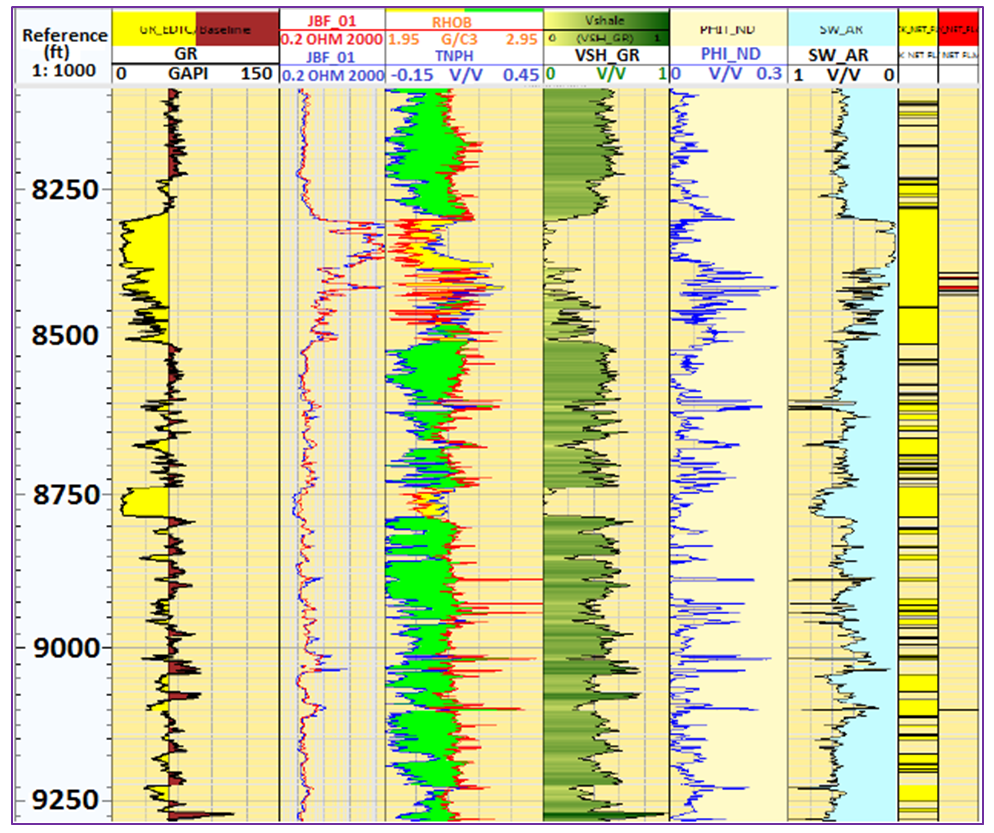 | Figure 4. Petrophysical well logs showing relevant parameters for the reservoir in the zone of interest |
 | Figure 5. Stratigraphic correlation of well no. 1, 2, 3, and 4 |
4.2. Reservoir Characterization and Geostatistical Modeling
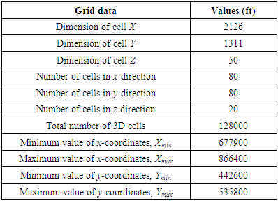
Characterization and modeling of complex clastic petroleum reservoirs has been the subject of intensive researches requiring the application of different techniques. Due to the high spatial heterogeneity of clastic systems, petroleum engineers face the common complications of providing reliable reservoir description. For this reason, detailed knowledge of reservoir properties is required to enhance description and facilitate hydrocarbon recovery processes. Therefore, analysing the spatial distribution pattern of reservoir properties to evaluate performance is an essential aspect of reservoir characterisation. Reliable characterisation of reservoir properties is the key elements for feasible economic evaluation of reservoirs. The provision of valuable information for characterising reservoir petrophysical properties facilitates the development and production of hydrocarbons and in consequence, the prediction of reserves in any oil or gas reservoir can be achieved (Islam et al., 2013). For the purpose of this research, geostatistical modeling approach has been used to build static reservoir models for porosity, permeability and thickness. Two conditional geostatistical methods and two other kriging methods are implemented in this section. These are sequential gaussian simulation, sequential indicator simulation, ordinary kriging and simple kriging. Comparative analysis of the two methods is performed. Validations on the generated models are done with available data using cross plots. Again, the spatial variability of the porosity, permeability and thickness is described in the subsequent chapters. Table 1 shows the summary of defined region of stationarity used in building the static reservoir models.Table 1. Grid data used in the static reservoir modeling
 |
| |
|
4.3. Spatial Analysis of Porosity, Permeability and Thickness
Certain variables of interest like porosity, permeability and thickness, among others are products that constitute the different chemical and physical processes in the oil and gas industry. It should be emphasized that the various physical and chemical processes superimposes the spatial configuration of the reservoir rock properties. Therefore, it is imperative to better understand the scales and directional perspectives of these variables in relation to hydrocarbon production. However, the spatial pattern of these variables at different well locations is very difficult to predict due to inherent geological uncertainties associated with their distribution. The fact that deterministic models do not take into consideration uncertainties; geostatistical modeling is recognized as an efficient approach. The probabilistic theory of geostatistical modeling captures uncertainties in reservoir property estimation. Mentioned earlier, geostatistical modeling is implemented in this study to describe the spatial variability of the porosity, permeability and thickness in the subsequent chapters.
4.4. Porosity from Ordinary Kriging
In this study, geostatistical conditional simulation is applied to model reservoir properties. The modeling of porosity was carried using ordinary kriging and sequential gaussian simulation. Generally, it is observed that the spatial-based map for porosity obtained from ordinary kriging is quite similar to the map generated from simple kriging. However, the ordinary kriging maps are slightly smoother in appearance compared to simple kriging maps. The estimated variance is larger in areas far from the data points and eventually becomes smaller in the grid blocks in areas close to the conditioning data. This is because ordinary kriging assumes a first-order stationary region which is strictly invalid at where the local mean is dependent on the sampled location. This leads to estimates that rely solely on neighboring girds, making a local average effect to produce smoother maps. The maximum variance for porosity estimated from ordinary kriging technique is 6.63, indicating minimal significant variations between the porosity dataset and estimated values. The minimum variance estimated from ordinary kriging method is recorded to be low as 0.73. The estimated porosity values from ordinary kriging ranged between 17.10% and 22.34% whereas the simulated map yielded high porosity values between 17.33 and 23.01%, respectively as seen in Figure 6(c). This shows a very high spatial continuity that can be observed from the various maps generated from ordinary kriging technique. All the data points spread significantly around the sample data that was used in populating the porosity flow unit data via ordinary kriging. The minimum and maximum values are closely related with few significant discrepancies. The porosity distribution profiles presented in Figure 6(a) to (c) is consistent with the well locations, indicating symmetric distributions across the field. Overall, the ordinary kriging maps showed good spatial continuity which trends from the east to the west directions of the reservoir. However, it is extremely difficult to detect the real distribution of each property variable based on visual inspection. More especially, the distribution for the variables may look differently based on the different number of bin chosen. As it can be seen in Figure 6(c), the sequential simulation gaussian map provided local variability to simulate reality for the porosity data to create equiprobable realizations (images). Four realizations were generated for porosity to describe its spatial distribution. The grid values of the maps generated from ordinary kriging are relatively different in appearance from the gaussian simulation map since the gaussian assumes a continuous normal distribution. As a result, the simulated map is not smoother compared to the map obtained from ordinary kriging method. The porosity distribution trend is very high from the middle to the west portions of the reservoir across the simulated map. Figure 6 shows the porosity distribution maps generated from ordinary kriging, ordinary kriging variance and sequential gaussian simulation.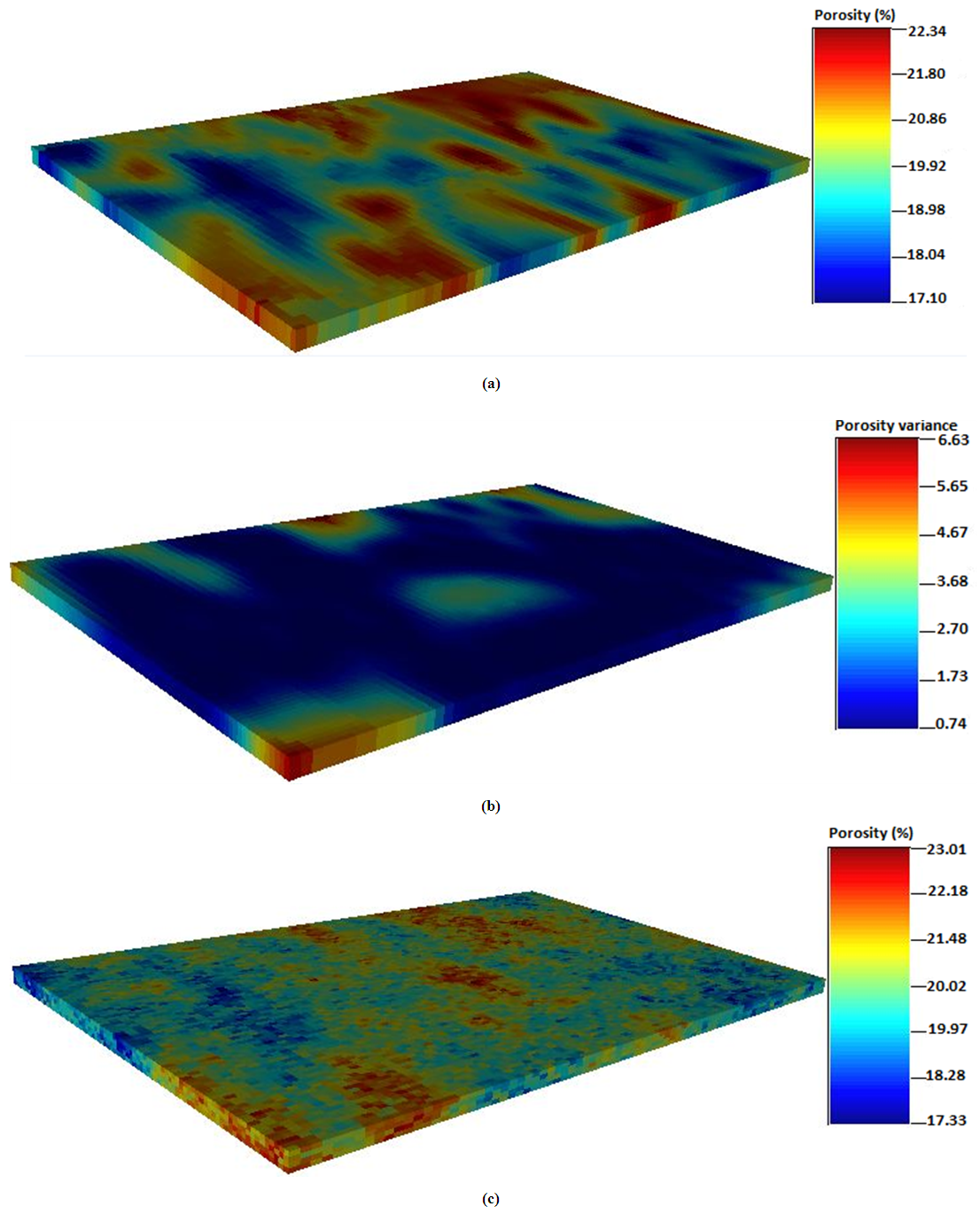 | Figure 6. Spatial distribution maps for porosity; (a) Ordinary kriging (b) Ordinary kriging variance (c) Sequential gaussian simulation |
4.4.1. Porosity from Simple Kriging
Simple kriging method is considered for porosity estimation and sequential gaussian simulation performed to subsequently generate multiple equal probable realizations. The simple kriging map presented in Figure 7(b) shows few significant variances for the porosity data. This is an indication of less error estimate for porosity values at unsampled location. The simulated map for porosity in Figure 7(c) showed good spatial continuity. The overall continuity of the simulated map is very high across the locations of the studied wells compared to the ordinary kriging. The good spatial continuity of the simple kriging map trends from east to the west corner of the reservoir. It recorded minimum and maximum porosity values of 17.21% and 23.12%. This suggests that simple kriging tends to over-predict properties of the reservoir. The estimation variance in the grid blocks is small as 0.72 and significantly large as 4.08. It should be mentioned that, simple kriging does not necessary reproduce extreme values of a property when populated within a grid block. Generally, symmetrical distribution is observed for simple kriging maps. It captured spatial structure for the flow unit porosity data. Due the scarcity nature of the sampled data, relatively small variation within the sampled data is observed. The variance for simple kriging map was much lower (i.e., 4.08) compared to ordinary kriging (i.e., 6.63). Next, four realizations (model descriptions) were generated for porosity using sequential gaussian simulation. Comparatively, it is observed that the estimated values are quite smaller than the sampled data. There are high porosity values spreading across the north-east location of the reservoir. However, we observed high simulated values for porosity than either of the two kriging techniques. The sequential gaussian simulation turned the porosity values into normal transform univariate distribution, scaled the raw data to unit sill and generated spatial-related values for porosity. However, there are no significant differences in terms of appearance for the spatial-based maps generated from both simple and ordinary kriging methods. Figure 7 shows the porosity distribution maps generated from simple kriging, simple kriging variance and sequential gaussian simulation. 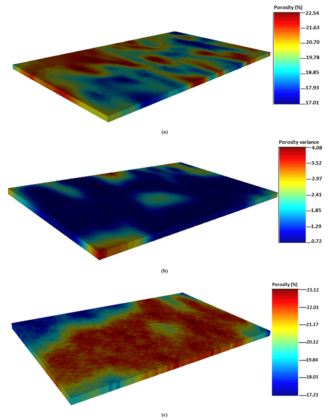 | Figure 7. Spatial distribution maps for porosity; (a) Simple kriging (b) Simple kriging variance (c) Sequential gaussian simulation |
4.5. Permeability from Ordinary Kriging
The spatial distribution maps for permeability are generated from ordinary kriging and sequential indicator simulation method. The permeability distributions are presented as log transforms of the actual sampled data. The simulated permeability values range from 3.05 (1122 mD) to 3.49 (3090 mD). The distribution for permeability shows a symmetric trend because the permeability values are clustered at one end. High permeability values are observed at the north east and south west corners of the grid model. Overall, the distribution of permeability across the reservoir grid showed a very good lateral continuity. The permeability map obtained from ordinary kriging estimation showed high spatial variations. The estimated values of permeability from ordinary kriging had low and high values of 3.01 (1023 mD) and 3.48 (3020 mD). The estimation variance for permeability is close to conditioning data. The distribution pattern is relatively higher at the central portion of the grid block. In this case, the conditioning data becomes extremely larger in the region far from the sampled data points. This suggests that the permeability distribution experienced a narrower spread than the conditioning data. However, the permeability distribution from the ordinary kriging method follows normal distribution trend. This implies that, the data points are distributed close to the estimated mean value. Figure 8(b) shows the variance map for permeability. The minimum and maximum variances are obtained as 0.11 and 1.23, respectively. In special cases where the sampled data becomes close to the conditioning data, the kriging variance becomes a reflection of the nugget of the variogram. In general, the ordinary kriging method provided good estimates for permeability distribution at well locations. It captured the spatial correlation at well locations in the permeability dataset. Figure 8 shows the spatial distribution maps for permeability obtained from ordinary kriging, ordinary kriging variance and sequential indicator simulation. 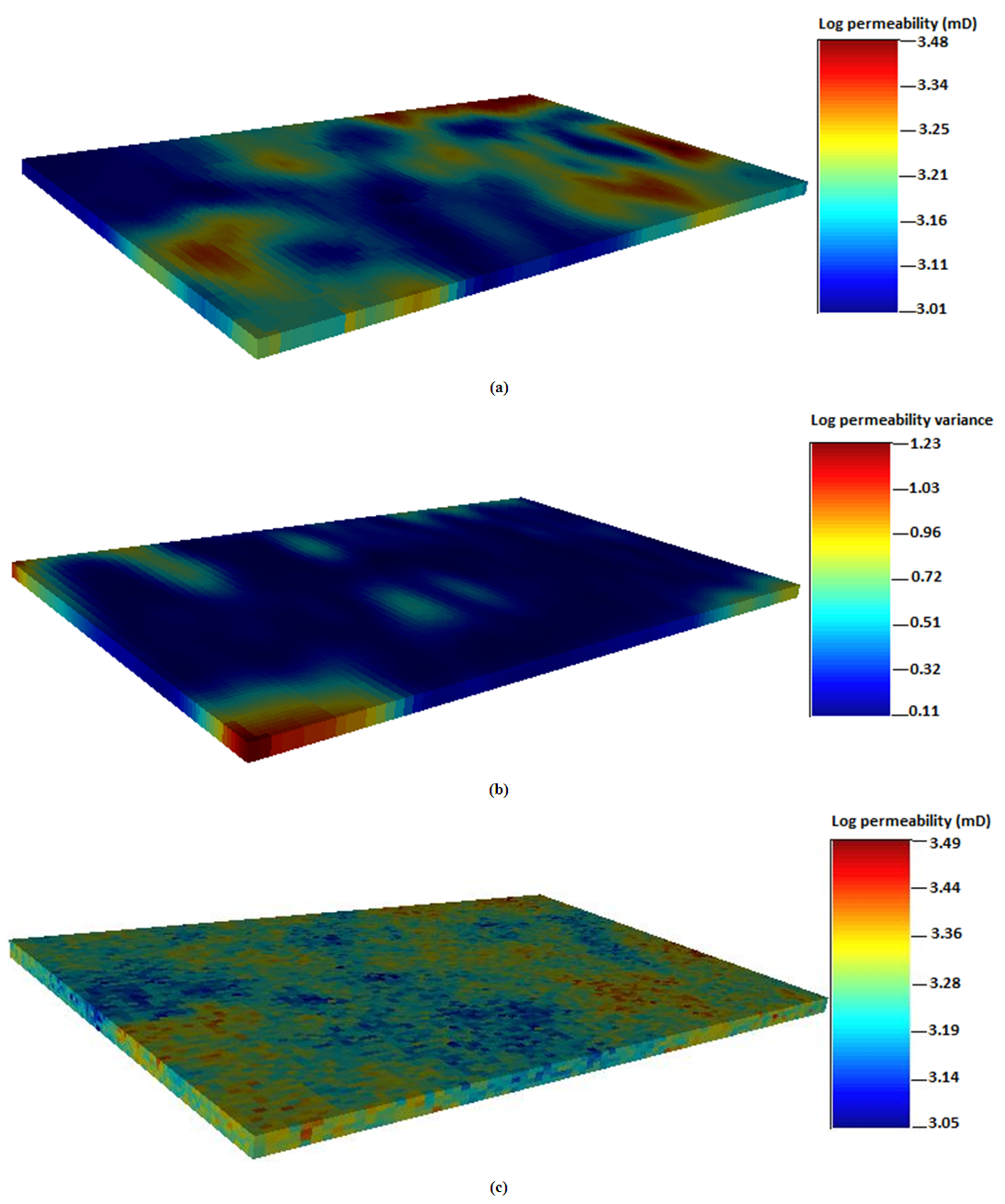 | Figure 8. Spatial distribution maps for permeability; (a) Ordinary kriging (b) Ordinary kriging variance (c) Sequential indicator simulation |
4.5.1. Permeability from Simple Kriging
Simple kriging and sequential indicator simulation were used to populate the permeability values at well locations. In all, the permeability distribution maps generated from both simple kriging and ordinary methods showed similar appearances. However, the maps from simple kriging technique were quite smoother in appearance compared to the ordinary kriging. Also, high values of permeability were obtained from the simple kriging. The simulated permeability values from simple kriging method peaked at 3.55 (3548 mD) whereas ordinary kriging recorded high permeability value of 3.49 (3090 mD). The simple kriging estimates for permeability ranged between 2.20 (158 mD) and 3.32 (2089 mD). The overall discrepancies for both techniques is very small as 0.16. This means that the estimation differences between both kriging methods are in proximity to each other. The estimated variance for permeability values tends to be higher at the extreme ends of the reservoir grid as shown in Figure 9(b). The estimation variances are between 0.08 and 1.19. This explains that the error variance for simple kriging is quite smaller than ordinary kriging. More importantly, both simple and ordinary kriging methods gave good estimates. However, estimation from simple kriging method appears to be closer to the conditioning data than ordinary kriging method. As seen in Figure 9(a), the blue region of the map represents areas where the true permeability values are found. Extending to the north east corner of the map, it is observed that predicted values from the simple kriging are much higher at these locations. This also the case for locations where the sampled data are much populated in the grid. This is because simple kriging distributes property data close to the mean value. Consequently, the simulated map for permeability is associated with extreme values. This could eventually reflect the intrinsic characteristics of the reservoir under consideration as four realizations were generated to capture the overall description of the reservoir. The simulation results in Figure 9(c) achieved a better spatial structure to describe the reservoir heterogeneity, although showed similar appearance to the kriging map presented in Figure (a). The simulation uses extreme values within the search neighborhood of the dataset unlike kriging which only utilizes values around the sampled location to predict the unsampled locations. Figure 9 shows the permeability distribution maps generated from simple kriging, simple kriging variance and sequential indicator simulation.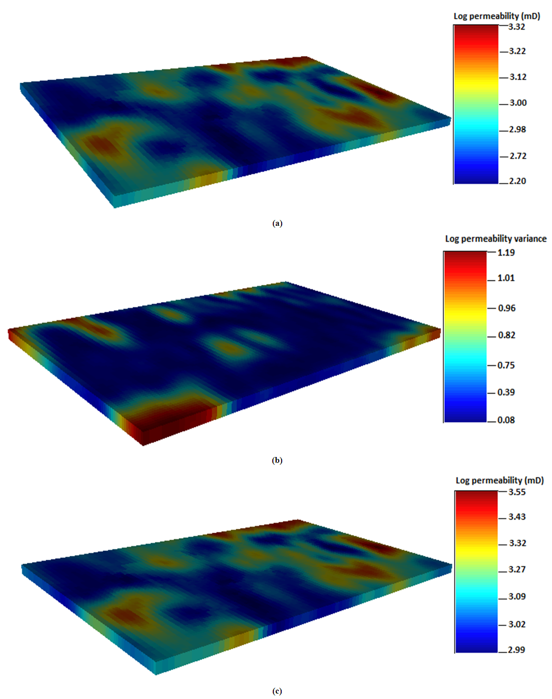 | Figure 9. Spatial distribution maps for permeability; (a) Simple kriging (b) Simple kriging variance (c) Sequential indicator simulation |
4.6. Thickness from Ordinary Kriging
The gross thickness for the reservoir is distributed within the grid model using ordinary kriging and sequential gaussian simulation as observed from Figure 10. The continuity of the thickness map generated from ordinary kriging is pretty similar to the simple kriging map. It shows high spatial continuity at the locations close to the sampled data. The data is highly distributed close the center locations through the entire maps. The estimated gross thicknesses from ordinary kriging are between 9.85 ft and 29.01 ft. However, there are few significant variations at the location where the various wells are distributed. The maximum value for estimated thickness is 37.80 ft whereas the maximum value for thickness data is 38.15 ft. The thickness data are populated with extreme values more than 10.12 ft. This shows no tremendous improvement of the conditioned data for thickness prediction. The estimation variances for thickness were low and high as 6.45 ft and 13.49 ft. In the north east corner of the grid, the thickness data is almost partitioned at the sub areas. High thickness values are observed for the sub areas of the ordinary kriging map. This can be seen in Figure 10(a). The maps generated from ordinary kriging shows good lateral continuity from the center to the west portions. This indicates relatively small variations in the thickness dataset. The small variations in the thickness distribution maps show closeness of the sampled data to the conditioned data. The thickness data followed normal distribution trend such that most of the sampled data were distributed close to the mean value. Overall, the thickness distribution maps showed some level of smoothness in appearance compared to the simple kriging maps. High thickness locations are observed from the simulated map shown in Figure 10(c). On the more note, it should be mentioned that the simulated thickness values were pretty higher than the two kriging estimations. Noticeably in Figure 10(c), simulated thickness values is much distributed at the extreme ends and spread continuously from the west to the east portion. However, the estimation variance becomes large at the northwest corner of the grid. The red and yellowish sections show areas with high thickness values. These are areas with good spatial continuity for gross thickness. The blues portions represent areas with low thickness values. Figure 10 shows the thickness distribution maps generated from ordinary kriging, ordinary kriging variance and sequential gaussian simulation. 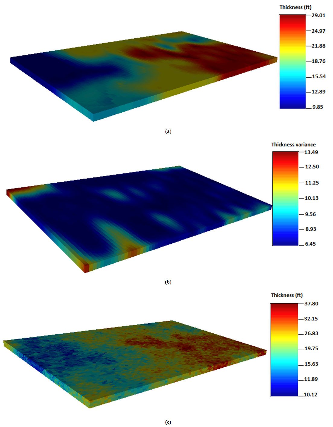 | Figure 10. Spatial distribution maps for thickness; (a) Ordinary kriging (b) Ordinary kriging variance (c) Sequential gaussian simulation |
4.6.1. Thickness from Simple Kriging
Thickness is further estimated from simple kriging and sequential gaussian simulation. Typically of simple kriging, the generated maps are quite smooth in appearance. It shows good spatial correlation (continuity) from the west to the east direction of the grid. Configuration of the conditioned data resulted in the west/east trend observed from the simple kriging map shown in Figure 11(a). The thickness data is distributed such that the conditioning data is undersampled within the search neighborhood relative to the other section of the grid. This area tends to have smaller variance for gross thickness values, indicating a better estimation result compared to ordinary kriging method. However, the maps generated from both kriging methods are pretty similar in physical appearance. The simple kriging variance map is shown in Figure 11(b). The estimated variances for thickness obtained from simple kriging are 7.56 ft and 14.01 ft. Close to the conditioning data, the estimation variance for thickness becomes extremely small in the gridblock. However, it becomes large in the sections far from the conditioning data. Consequently, sequential gaussian simulation map captured intrinsic characteristics of the field, although it could not estimate the exact distribution of each populated variable defined within the grid block. 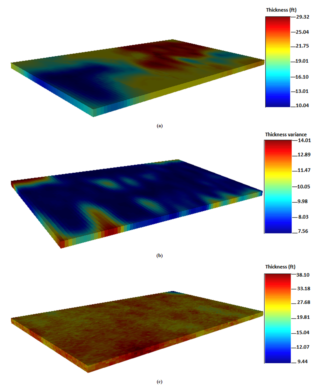 | Figure 11. Spatial distribution maps for thickness; (a) Simple kriging (b) Simple kriging variance (c) Sequential gaussian simulation |
On the more note, the simulated map presented in Figure 11(c) revealed high thickness values between 9.44 ft and 38.10 ft. The thickness data is distributed uniformly at the northwest corner portion of the grid model. The blue section represents areas with low thickness values while the red and yellowish portions represent areas with high thickness values. The simple kriging method yielded low and high thickness values of 10.04 ft and 29.32 ft. It predicted thickness values that are much larger than the estimated mean value. That is 19.9 ft. Because simple kriging does not produce values close to extreme values for spatial-related data, the thickness data modeled in this study showed a narrow spread close to the sampled data. The maximum value for thickness data is 23.12 ft whilst the maximum estimated value from simple kriging is 29.32 ft. It should be mentioned that the distributions for thickness are consistent with location of the wells under consideration. This brings the idea that the thickness distributions are representative of the different well profiles. Figure 11 shows the thickness distribution maps generated from simple kriging, simple kriging variance and sequential gaussian simulation.
4.7. Ranking of Geostatistical Reservoir Models
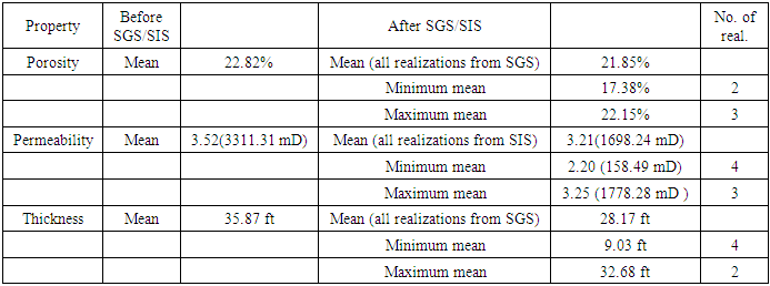
Four equiprobable realizations were generated for porosity, permeability and gross thickness and ranked. The ranking involved comparing the statistical mean values for each of the reservoir properties modeled, before and after the various simulations. The ranking is performed for the different property realizations by comparing mean values from the raw data used with the mean values from simulated data. The significant variations in the minimum and maximum mean values after the ranking process provided ideas of what the geostatistical models are well represented in the studied reservoir. Consequently, geostatistical modeling predicted values that are smaller than the real field data after the simulation. This observation can be seen in Table 2. Generally, the mean values of the simulated data become slightly smaller than the mean values of the raw data. The possible reason behind this observation is attributed to the variations incurred in the minimum and maximum parameters of each property used in the variogram computation. This implies that generating multiple realizations for porosity, permeability and thickness are reliable method for enhanced reservoir characterization. The method minimizes uncertainties related with petrophysical property estimations. Table 2 shows summary of statistical parameters from the geostatistical ranking.Table 2. Summary of geostatistical ranking for realizations of properties
 |
| |
|
4.8. Statistical Analysis and Variography
Statistical analysis is performed for porosity, permeability and thickness. Total number of 4,200 data points was used as the input values for the analysis. Semi variograms were fitted for each property to infer the spatial variability between the sampled data point as a function of distance and location. The core mandate of the statistical analysis was to evaluate the behaviour of the distribution pattern of the input variables (i.e., porosity, permeability and thickness). However, it is not an easy task to interpret large numbers of raw data points from oil reservoirs in the digital format from geostatistical perspective. Therefore, the raw data was well-organized and analyzed critically using univariate statistical analysis. The various parameters are summarized and presented in the form of tables, charts to provide vivid picture of their variations in the reservoir under consideration. From this point of discussion, it can be stated that statistical analysis is an essential aspect of geostatistical modeling commonly used for quantifying reservoir heterogeneity. Noted earlier, the descriptive univariate analysis provided several statistical parameters to gain insight for describing distribution trend of the dataset used. Also, the different statistical parameters were computed. These included the mean, median, minimum, maximum, variance, standard deviation, lower and upper quartiles and coefficient of variation. Statistical parameters like the mean, median, and coefficient of variation can determine the type of distribution. The median and mean statistical parameters provide information about the central location for mass property distributions whereas the standard deviation and variance describe the spatial correlation (variability) of the input data.
4.8.1. Statistical Analysis and Variography for Porosity
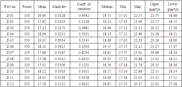
Descriptive statistics is performed for porosity and variogram computed. The spatial variability for the porosity data points was described in the omnidirectional variogram model. It is assumed that the direction of minimum and maximum of the selected variogram are at right-angles to each other. That is 90°. Exponential variogram model was fitted by visual inspection to populate the porosity data as shown in Figure 12(a). The input variables used for variogram analysis of porosity is described as follows. The minimum, median and maximum ranges for porosity data are 3600 ft, 18800 ft and 35600 ft. Lag separation of 50 ft was used. The number of lags used in calculating the variogram is 65. The nugget effect and the sill contribution values are 6.7 and 20.3. The tolerance of direction is 90 ̊. The lag distance (tolerance of distance) and allowable bandwidth are 105 ft and 1800 ft. Anisotropic effect was taken into consideration in the variogram analysis to ensure symmetric continuity. Therefore, azimuth and dip angle of 180° and 90° were used. Moreover, histogram plot is generated for porosity data using bin width of 12, respectively. This is shown in Figure 12(b). It is observed that the frequency of each bin from the histogram decreases with increase in bin number. This is as a result of reduction in bin length. The mean and median porosity values from the histogram plot for the entire reservoir are 19.90% and 19.75%, and the minimum and maximum values are 17.01% and 22.54%. The mode is around 22%. High coefficient of variation value of 0.4042 is obtained for the porosity data points. The least deviation is around 0.0014 and the variance is 2.91. This signifies appreciable level of prediction for porosity. Figure 12 shows the variogram model and histogram plot for porosity. Table 3 presents the statistical variables for porosity.Table 3. Statistical analysis for porosity of the wells in the reservoir
 |
| |
|
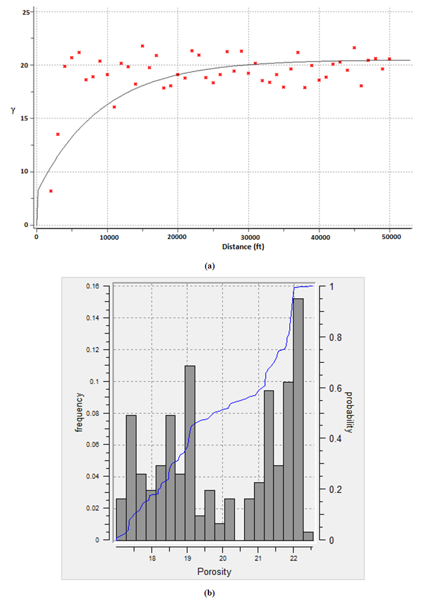 | Figure 12. Porosity; (a) anisotropic variogram model (b) histogram plot |
4.8.2. Statistical Analysis and Variography for Permeability
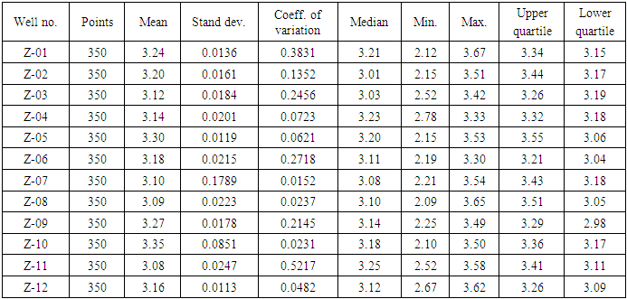
Statistical analysis is subsequently performed for permeability and corresponding anisotropic variogram calculated. Omni-directional gaussian variogram model was fitted to distribute the permeability data as shown in Figure 13(a). Key input parameters used for the variogram computation included: nugget effect, sill contribution, range, tolerance limit, lags distance, azimuth, dip angle and bandwidth. The minimum, median and maximum ranges for the permeability data are 500 ft, 1975 ft and 3900 ft. The lag separation is 40 ft, and the number of lags is 85. The nugget effect and sill contribution values of the variogram model are 1.15 and 4.38. The tolerance of direction is 90°. This was used to cater for the effect of anisotropy to ensure symmetric continuity in the permeability distribution. Azimuth and dip angle values of 180° and 90° were specified to populate the permeability data. The lag distance (tolerance of distance) and acceptable bandwidth are 98 ft and 1700 ft. Histogram plot is generated for permeability using a bin width of 12, as shown in Figure 13(b) and descriptive statistics performed. It can be seen from Figure 13(b) that, the frequency of each bin for log transformed-permeability data decreased with increase in bin number and consequently reduces bin length. Overall, the median and mean values from the histogram for log permeability are 3.23 (1698 mD) and 3.25 (1778 mD). The modal value is around 3.21 (1621 mD). The least deviation and coefficient of variation values for log permeability are 0.0113 and 0.0152. The coefficient of variation describes the spread of extreme values from the sampled data. However, low values of coefficient variances were observed as shown in Table 4. This means there are no outliers in the estimation and hence, there is high validity for the permeability estimation. Figure 13 shows the variogram model and histogram plot for permeability data. Table 4 presents the statistical variables for log permeability. Table 4. Statistical analysis for log permeability of the wells in the reservoir
 |
| |
|
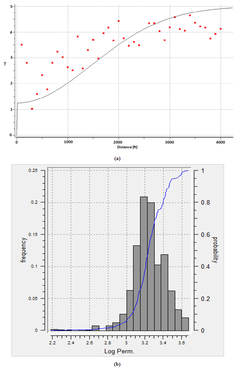 | Figure 13. Log permeability; (a) anisotropic variogram model (b) histogram plot |
4.8.3. Statistical Analysis and Variography for Thickness
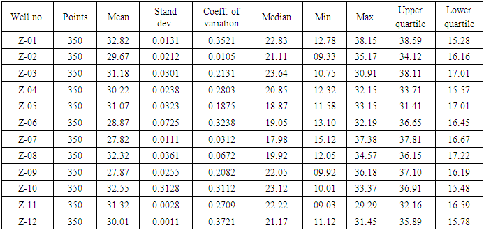
Statistical analysis is performed for thickness to understand their distributions. Anisotropic variogram is calculated and gaussian variogram model fitted for thickness data as shown in Figure 14(a). First, we assumed that the minimum and maximum continuity of directions of the variogram are perpendicular to each other. For this reason, omnidirectional variogram model is selected to cater for anisotropic effect in the estimation process. Because thickness is a discrete property which constitutes different replicated integers, the gaussian simulation transformed the data into continuous normal distribution for easy estimation. However, it should be mentioned that the structures of the variogram showed similar direction of continuity regardless of the input variables. Noticeably, it is very difficult to judge the different continuity of directions in the variogram by visual inspection. The nugget effect, sill contribution, ranges, tolerance limit, lag distance, azimuth, dip angle and bandwidth were used as major input properties for the variogram computation. Nugget effect and sill contribution values of the computed variogram for thickness are 3.5 and 33.80. The minimum, median and maximum ranges are 2200 ft, 4400 ft and 38000 ft. The lag tolerance is 112 ft, and the permissible lag separation is 45 ft. Bandwidth of 1670 ft is considered. The direction of continuity of the variogram model was given a tolerance of 90°, and an azimuth value of 180°, respectively. The angle of dip is 90°. Histogram is plotted for the thickness as shown in Figure 14(b). The thickness data is divided into 12 bins at varying bin lengths. The mean and median values for thickness observed from the histogram are 32.82 ft and 22.73 ft. The minimum and maximum values for thickness are 12.8 ft and 37.55 ft. High correlation coefficient value of 0.3721 is obtained for thickness distribution, indicating more valid estimation for thickness. The minimum deviation is estimated to be 0.0011. Figure 14 shows the variogram model and histogram plot for thickness data. Table 5 presents the statistical variables for thickness.Table 5. Statistical analysis for thickness of the wells in the reservoir
 |
| |
|
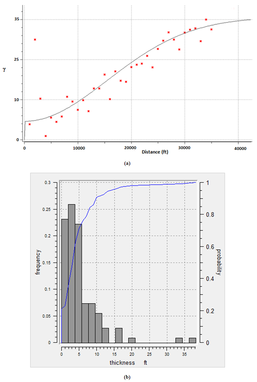 | Figure 14. Thickness; (a) anisotropic variogram model (b) histogram plot |
4.9. Regression Analysis and Model Validations
Detailed understanding of spatial distribution of data requires the need to draw Q-Q plots. In the Q-Q plot, the sampled data is compared to theoretical modeled distribution. To achieve the set objective of this paper, validation is performed between simulated (modeled) data and the estimated (kriging) data via the real field data. The results obtained are compared using cross plots as shown in Figure 15. The simulated data is plotted against actual and the estimated data after the quantile normal transformation. Quantile normalization line at 45° angle is established to check correlation between the real data and the predicted data for validation of the proposed gaussian and kriging models. The Q-Q type of plot ensures that the observed data points are well-fitted to the 45° line. The closer the data points to the 45° line, more validity for the generated models. In cases where the theoretical quantile exceed a value of one, the fitting becomes poor due to a phenomenon called tail effect or outliers. Generally, the gaussian predicted more details compared to the kriging methods. The relationship between the simulated data and real data for porosity, permeability and thickness showed less significant outliers as shown in Figure 15. However, the variables of interest (i.e., porosity, permeability and thickness data) are skewed to the either sides of the indicating a symmetric distribution called gaussian (normal) distribution. Gaussian distribution ideally predicted based on variance and mean of the input variables. Cross plot validations for the variables showed higher degree of compatibility of real data. This means that the predicted and simulated data were close to the 45° line and consequently depict more valid estimations for modeling generated. However, the sequential gaussian simulation method showed more compatibility with the real data for porosity, permeability and thickness, compared with kriging method. Figure 15 shows the model validations for porosity, permeability and thickness estimation from Q-Q plots.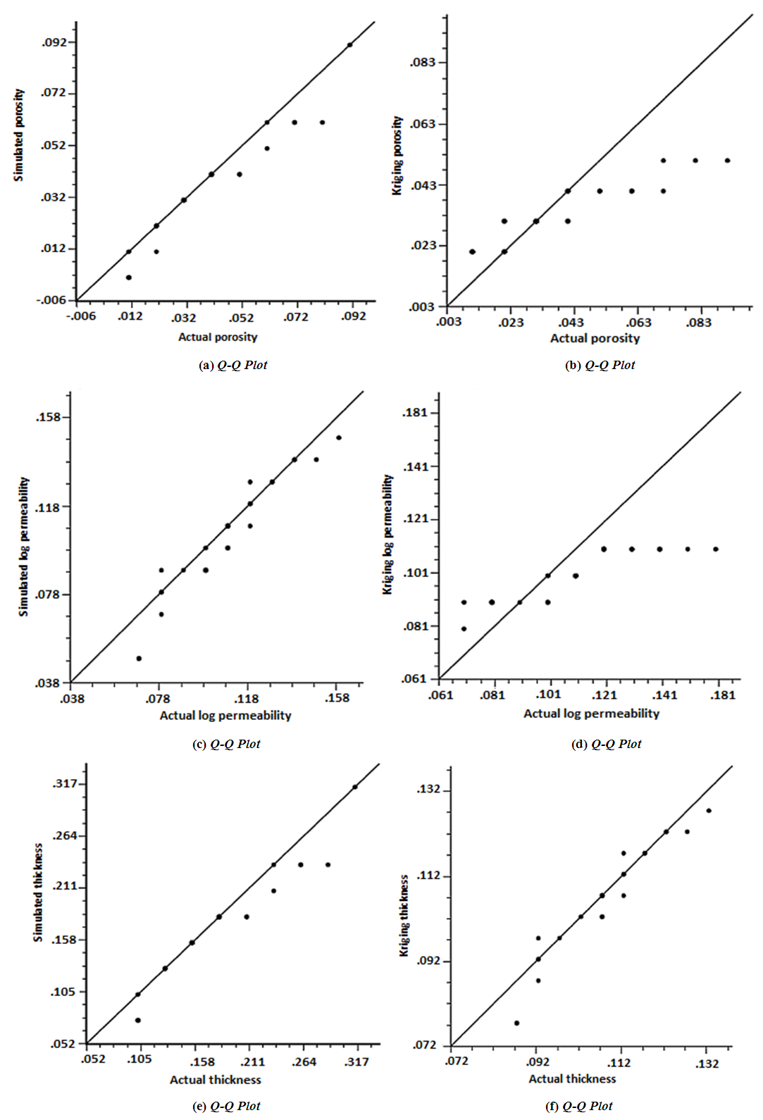 | Figure 15. (a) Cross plot validation between simulated data and real porosity data. (b) Cross plot validation between real porosity data and kriging-estimated data. (c) Cross plot validation between simulated data and real permeability data. (d) Cross plot validation between real permeability data and kriging-estimated data. (e) Cross plot validation between simulated data and real thickness data. (f) Cross plot validation between real thickness data and kriging-estimated data |
5. Conclusions
The study showed that: (i) porosity, permeability and thickness were largely distributed at the center towards north-east direction of the reservoir. This can be observed from the spatial-based maps. The kriging methods provided good estimates that described the variations of porosity, permeability and thickness in the reservoir. The porosity, permeability and thickness values estimated from simple kriging method ranges from 17.01 to 22.54%, 158.48 to 2089.29 mD and 10.04 to 29.32 ft. The ordinary kriging method predicted porosity, permeability and thickness values from 17.10 to 22.34%, 1023.29 to 3019.95 mD and 9.85 to 29.01 ft. However, the conditional simulation methods (sequential gaussian simulation and sequential indicator simulation) gave high porosity, permeability and thickness values, ranging from 17.21 to 23.12%, 977.23 to 3548.13 mD and 9.44 to 38.10 ft. The wide range of porosity, permeability and thickness values observed could describe the reservoir of having high storativity, flow capacity and good pay zones for oil and gas accumulations. (ii) The observed relatively dissimilarities between the kriging maps and the gaussian maps in terms of appearance is attributed to the fact that, the kriging methods tends to minimize error variance in estimation for smoother distribution of variables while gaussian simulation approach transformed error variance into probable variables to give details in the flow unit data for porosity, permeability and thickness predictions. Also, the kriging maps showed much transitional changes in subregions of the reservoir than the gaussian simulation maps. This is because the effect of order-of-magnitude variations and extreme girds within the flow unit dataset was minimized to obtain better images (maps) with good spatial structure that captured the significant variations of porosity, permeability and thickness for the case study. (iii) The anisotropic variogram analysis (variography) better explained the porosity, permeability and gross thickness distributions in the reservoir as a function of distance and location. Using the nugget effect, range and sill as key input parameters for variogram analysis has provided detailed information on potential locations for future oil drilling projects. (iv) Furthermore, the regression-based analysis evaluated reliability of the generated models. From this analysis, it is observed that more data points were closer to the quantile normalization line (i.e., 45° line), depicting more validity for proposed gaussian and kriging models. The univariate statistical analysis showed coefficient of variation values for porosity, permeability and gross thickness distributions as: 0.4042, 0.5217 and 0.3721, indicating less outlier and appreciable level of prediction for porosity, permeability and thickness. Conclusively, it can be stated emphatically that, geostatistical methods are efficient approach to describe reservoir heterogeneity. It has provided the means for describing the spatial distributions of porosity, permeability and thickness for performance evaluation of the Jubilee oilfield, Ghana.
ACKNOWLEDGEMENTS
The described article was carried out as part of the Scientific Research Initiative for All Nations University College (ANUC), Ghana. The research is supported by the Oil and Gas Engineering Department, School of Engineering - All Nations University College, co-financed by Mrs Mavis Annan Boah, Assistant Group of Companies, Italy.
References
| [1] | Abrokwah, B. Y.E. (2010). An Overview of Ghana’s Oil and Gas Disclaimer. Lecture Notes, University of Ghana. |
| [2] | Brownfield, M. E., and Charpentier, R. R. (2006). Geology and Total Petroleum Systems of the Gulf of Guinea Province of West Africa: U.S Geological Survey Bulletin 2207-c, p. 32. |
| [3] | Clark, I., (2000). Practical Geostatistics. Applied Science Publishers Ltd., London, pp: 129. |
| [4] | Clark I., (2001). Practical Geostatistics. Otterbein College, Columbus, Ohio, USA. pp 51-55. |
| [5] | Deutsch, C., Wang, L. (1996). Hierarchical Object Based Stochastic Modeling of Fluvial Reservoir. Mathematical Geology 28(7), pp. 857-880. |
| [6] | Deutsch, C. V. and A. G. Journel (1992). GSLIB: Geostatistical Software Library and User’s Guide, Oxford University Press, New York, 340 p. |
| [7] | Geoff B. (2007). S-GeMS Tutorial Notes, Kansas Geological Survey. |
| [8] | Goovaerts P. (1997). Geostatistics for Natural Resources Evaluation, Oxford University Press. |
| [9] | GNPC (1989). Petro-Canada International Assistance Corporation on the Stratigraphy of Offshore Ghana" An Unpublished Report. |
| [10] | Islam A.R.M.T, Habib, M. A, Islam, M.T and Mita M. R. (2013). Interpretation of Wireline Log data for Reservoir Characterization of the Rashidpur Gas Field, Bengal Basin, Bangladesh. Bangladesh Geoscience Journal, Volume 1, Issue 4, 47-54. |
| [11] | Johnston, K., Ver Hoef, J. M., Krivoruchko, K., and Lucas, N., (2003). The Principles of Geostatistical Analysis. Using ArcGIS Geostatistical Analyst. pp 49-80. |
| [12] | Journel, A.G. and Huijbregts, C.J. (1978). Mining Geostatistics. Academic Press, London, 600 p. |
| [13] | Journel A.G. and Alabert F., (1989). Non-Gaussian data expansion in the earth sciences Terra Nova 1 123–34. |
| [14] | Journel A.G. and Hernandez G. (1989). Stochastic Imaging of the Wilmington Clastic Sequence SPE 19 857. |
| [15] | Kastning T. (2012). Basic Overview of Ghana’s Emerging Oil Industry. Published Report for Friedrich Ebert Stiftung (FES): 1–20. |
| [16] | Kelkar, M. and Perez, G. (2002). Applied Geostatistics for Reservoir Characterization. Society of Petroleum Engineers, Richardson, Texas, 30-50. |
| [17] | Kelkar, M., Perez, G., and Chopra, A. (2002). Applied Geostatistics for Reservoir Characterization. Richardson, TX: Society of Petroleum Engineers. pp 103. |
| [18] | Kelsall J. and Wakefield J. (2002) Modeling Spatial Variation in Disease Risk. J Am Stat Assoc 97(459):692-701. |
| [19] | Krige, Danie G. (1951). A Statistical Approach to Some Basic Mine Valuation Problems on the Witwatersrand. J. of the Chem., Metal. and Mining Soc. of South Africa. 52 (6): 119–139. |
| [20] | Lake, L. W., Liang, X., Edgar, T.F., Al-Yousef, A., Sayarpour, M., and Weber, D. (2007). Optimization of Oil Production Based on a Capacitance Model of Production and Injection Rates. In Hydrocarbon Economics and Evaluation Symposium. Society of Petroleum Engineers. |
| [21] | Matheron G, Beucher H, de Fouquet Ch, Galli A, Guérillot D and Ravanne Ch. (1987). Conditional Simulation of the Geometry of Fluvio-Deltaic Reservoirs SPE 16753. |
| [22] | Mpanza M. (2015). A Comparison of Ordinary and Simple Kriging on a PEG Resource in the Eastern Limb of the Bushveld Complex. Johanesberg. pp 25 – 30. |
| [23] | Perez, V. S. and A. G. Journel., (1990). Stochastic Simulation of Lithofacies for Reservoir Characterisation, In Report 3, Stanford Center for Reservoir Forecasting, Stanford, CA. |
| [24] | Pyrcz, M. J. and Deutsch C. V. (2014). Geostatistical Reservoir Modeling. Oxford University Press. |
| [25] | Remy N. (2004). Geostatistical Earth Modeling Software: User’s Manual. |
| [26] | Remy Nicolas, Alexander Boucher and Jianbing Wu. (2009). Applied Geostatistics With SGEMS, A User’s Guide. Cambridge University Press UK. pp 66-67. |
| [27] | Srivastava R.M, Frykman P., Jensen M. (2004). Geostatistical Simulation of Framework Networks, Geostat Banff 2005:295-304. |
| [28] | Tullow (2013). Report of the External Monitoring Group Prepared for International Finance Corporation, Jubilee Project. Tullow Oil Limited, Accra, Ghana. Retrieved 22 April 2013. |
| [29] | Wilson C.E, Aydin A, Durlofsky L.J, Boucher A., Brownlow D.T. (2011). Use of Outcrop Observations, Geostatistical Analysis and Flow Simulation to Investigate Structural Control on Secondary Hydrocarbon Migration in the Anacacho Limestone, Uvalde, Texas. AAPG Bull 95(7): 1181-1206. |
| [30] | Zarei A, Masihi M, Salahshoor K . (2011). Comparison of Different Univariate and Multivariate Geostatistical Methods by Porosity Modeling of an Iranian Oil Field. Pet Sci Technol 29(19): 2061-2076. |
| [31] | Zhao Shan, Yang Zhou, Mengyuan Wang, Xiaying Xin and Feng Chen. (2014). Thickness, Porosity, and Permeability Prediction: Comparative Studies and Application of the Geostastical Modeling in an Oil field. Environmental Research Systems 3:7. |

 Abstract
 Reference
 Full-Text PDF
 Full-text HTML