1. Introduction

Earthquake occurs in a cyclic order. From regular observations it is known that two major seismic events are usually separated by a comparatively long aseismic period. In this aseismic period observations show slow surface movements, indicating a slow aseismic change of stress and strain in the vicinity of the fault. In this paper we developed a theoretical model of lithosphere-asthenospohere system represented by three layered elastic half-space. Such theoretical models was considered by Sato [1], Rybicki [2, 3], Mukhopadhyay [4, 5], Mukherjee [6], Sen and Debnath, [7], Debnath and Sen [8-10], Debnath and Sen [11-13], Mondal and Sen [14].

2. Formulation

We consider a theoretical model of lithosphere-asthenosphere system consisting of two elastic layers and a elastic half-space. The layers and half-space are assumed to be in welded contact. The depth of the boundaries of two layers from free surface is taken as and second layer and half-space as We consider a buried vertical strike-slip fault situated in the second layer and the length of the fault is very large compare to its width The depth of the upper edge of the fault below the boundary of two layers is and upper and lower edges of the fault are horizontal. We introduce a rectangular Cartesian co-ordinate system with the plane free surface as the plane is taken vertically downwards in the medium, is taken along the strike of the fault on the free surface.

The boundaries between two layers and second layers and half-space are given by respectively. For convenience of analysis we introduce another set of Cartesian co-ordinate system with the upper edge of the fault is taken as and the plane of the fault is taken as the plane so that the fault is given by 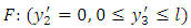. The relations between two co-ordinate system are given by

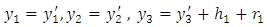(1)

The first elastic layer, the second elastic layer and elastic half-space are represented by and respectively. The Figure 1 shows the section of the theoretical model by the plane

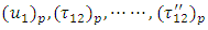
It is assumed that the length of the faults are large compared to their depths. So the displacements, stresses and strains are independent of and depend only on Then the components of displacement, stress and strain can be divided into two groups, one associated with strike-slip movement and another associated with dip-slip movement of the fault. Since in this model the strike-slip movement of the fault is considered, then the displacement, stress and strain components associated with long strike-slip fault for two layers and half-space are and respectively.

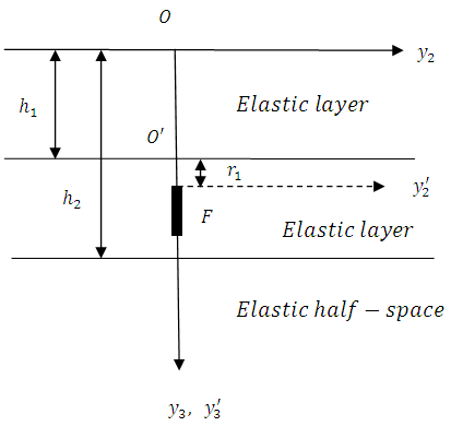Figure 1. Section of the model by the plane

2.1. Constitutive Equations (Stress-Strain Relations)

For the first elastic layer, the stress-strain relation can be written in the following form:

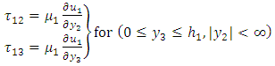(2)

where is the rigidity of the first elastic layer.

For the second elastic layer, the stress-strain relation can be written in the following form:

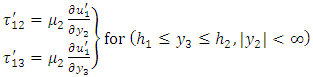(3)

where is the rigidity of the second elastic layer.

For half-space, the stress-strain relation can be written in the following form:

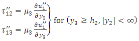(4)

where are rigidity of the half-space.

The rigidities of the elastic layers and half-space are assumed to be constant.

2.2. Stress Equation of Motion

For a slow, aseismic, quasi-static deformation the magnitude of the inertial terms are very small compared to the other terms in the stress equation of motion and they can be neglected. Hence relevant stress satisfy the relations:

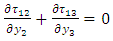(5)

for the first elastic layer

(6)

for the second elastic layer

(7)

for the elastic half-space

From equation (2)-(7) we get

(8)

(9)

(10)

2.3. Boundary Conditions

We assume that the upper surface of the first elastic layer is stress-free and the two layers and the second layer and half-space are assumed to be in welded contact. Then the boundary conditions are given below

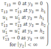(11)

2.4. Initial Conditions

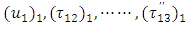
We assume that the time t is measured from a suitable instant when the model is in aseismic state and there is no seismic disturbance in it. are the values of at time and they satisfy all the relations stated above.

2.5. Conditions at Infinity

At a large distance from the fault plane there is a shear strain which may changes with time maintained by the tectonic forces. Then

(12)

(13)

(14)

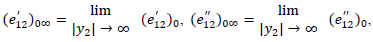where where 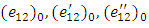are the values of at time In the medium of lithosphere-asthenosphere the layers and half-space are in welded contact, same has been taken for each layer and half-space, since strains are continuous at the boundaries of layers. From the major earthquakes it has been observed that the stresses release may be of the order of 400 bars. Keeping this in view, if we take to be linearly increasing function of time t with If we take then the value of should be of the order of

3. Displacements, Stresses and Strains in the Absence of Fault Movement

To obtain the solution for displacements, stresses and strains in the absence of fault movement we solve the boundary value problem (2)-(14) and get the solution in the following form:

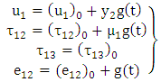(15)

for the first elastic layer

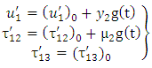(16)

for the second elastic layer

(17)

for the half-space.

4. Displacements, Stresses and Strains after the Restoration of Aseismic State Following a Sudden Strike-Slip Movement across the Fault

It is to be noted that due to a sudden fault movement across the fault the accumulated stress will be released to some extent and the fault becomes locked again when the shear stress near the fault has sufficiently been released. The disturbance generated due to this sudden slip across the fault will gradually die out within a short span of time. During this short period, the inertia terms can not be neglected, so that our basic equations are no longer valid. We leave out this short span of time from our consideration and consider the model afresh from a suitable instant when the aseismic state re-established in the model. We determine the displacements, stresses and strains after the fault movement with respect to new time origin So that all the equations (2)-(14) are also valid.

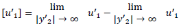
The sudden movement across is characterized by the discontinuity of across is defined as

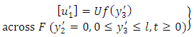(18)

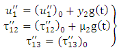
where and is a continuous function of and U is constant, independent of and . All the other components are continuous everywhere in the medium.

We try to obtain the displacements stresses for (with respect to new time origin) due to the movement across F in the following form:

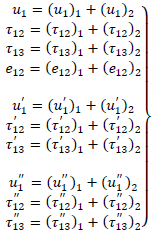(19)

where satisfy all the equations (2)-(14) and continuous throughout the medium. While 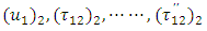satisfy all the relations (2)-(11) and also the dislocation condition (18) together with

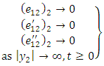(20)

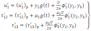
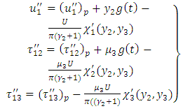
Then the solutions for are given by

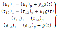(21)

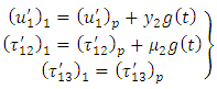(22)

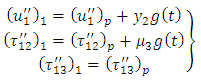(23)

where are the values of 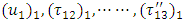respectively at (i.e. new time origin).

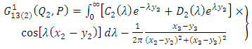
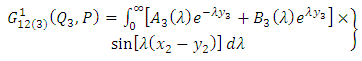
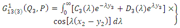
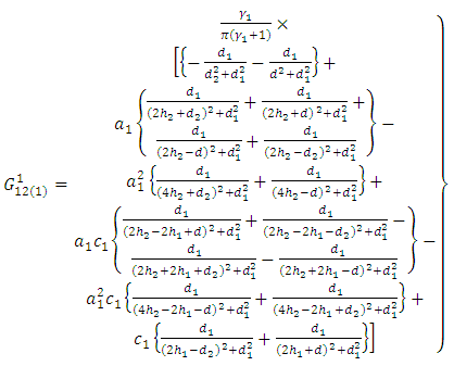
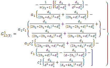
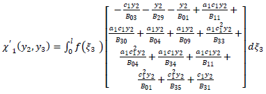
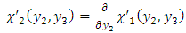
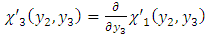
Now to solve the boundary value problem containing 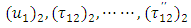we use Green’s function technique developed by Maruyama [15] and Rybicki [2, 3] as explained in Appendix. The required solutions are obtained as

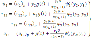(24)

for the first elastic layer

(25)

for the second elastic layer

(26)

for the half-space.

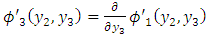
where and analytical form of are given in Appendix.

It is found that the displacements, stresses and strains will be finite and single valued any where in the model if the following conditions are satisfied

(i) and are both continuous functions of

(ii) f(0) = 0, f(l) = 0 and

(iii) Either is continuous in or is continuous in except for a finite number of points of finite discontinuity in is continuous in except possibly for a finite number of points of finite discontinuity and for the end points of (0, l), there exist real constant m, n both < 1 such that or a finite limit as and or to a finite limit as

5. Numerical Computations

To study the surface displacements, stresses and strain accumulation/ release and the shear stress near fault tending to cause strike-slip movement as we choose is the width of the fault . from free surface, representing the upper part of the lithosphere and upper part of the asrhenosphere.

We take , U = 40 cm, is the slip across F and for the function.

It is assumed that due to some tectonic reason there is a slow but steady accumulation of shear strain at a distance far away from the fault. Keeping this in view we take g(t) to be linearly increasing with time and g(0) = 0. With this assumption, we take g(t) = kt. From major earthquakes it has been observed that the stress release may be of the order of 400 bars. So we assume noting also that the observed rate of strain accumulation in seismically active regions during the aseismic period is of the order of to per year.

The values of model parameters are taken from the book of Aki [16], Cathles [17], Bullen and Bolt [18] and research papers by Clift [19], Karato [20]. We now compute the following quantities

(i) The residual/ additional surface shear strain due to fault slip near the fault after restoration of aseismic state

(ii) Change in shear stress in the first layer due to fault movement.

(ii) Change in shear stress in the second layer due to fault movement.

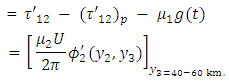The change in surface shear strain with near fault after restoration of aseismic state is shown in Figure 2. The figure shows that the fault movement leads to release of the surface shear strain and the effect is symmetrical about the fault trace. The magnitude of this shear strain release is maximum near fault trace and then falls off rapidly as we move away from the fault and become very small for large value of

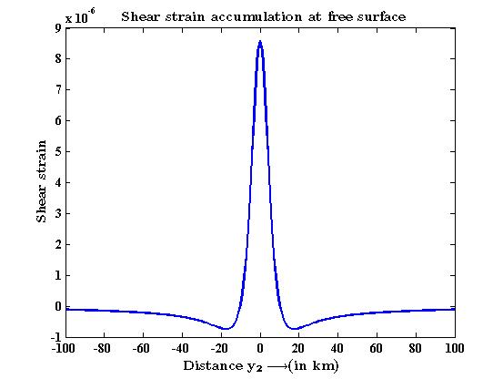Figure 2. Surface shear strain due to fault movement

The Figure 3 and 4 shows the contour map in the first and second layer respectively due to fault movement across the fault F after restoration of aseismic state.

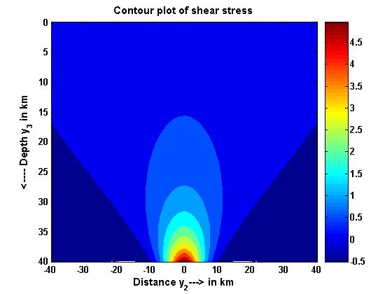Figure 3. Contour map of shear stress in the first layer

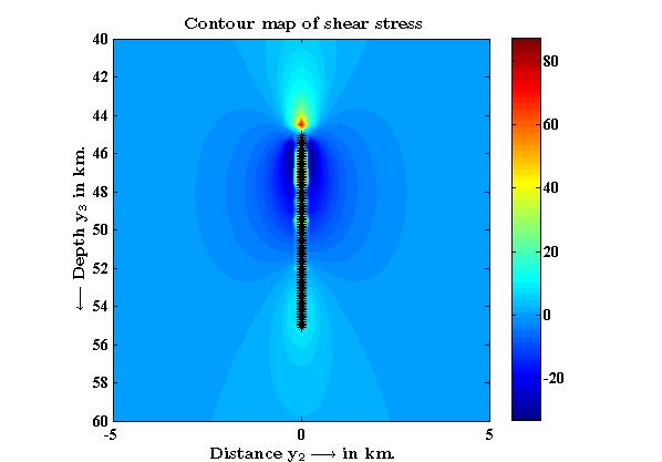Figure 4. Contour map of shear stress in the second layer

6. Conclusions

It is observed that the movement across the fault system significantly effect the nature of stress accumulation in the region. The rate of accumulation of stress in the system after the fault movement may give us some idea about the time to the next major event. Such results may be used for the purpose of prediction of earthquakes.

ACKNOWLEDGEMENTS

One of the authors Asish Karmakar thanks the Head Master of Udairampur Pallisree Sikshayatan (H.S.) for allowing me to pursue the research, and also thanks the Geological Survey of India; Department of Applied Mathematics, University of Calcutta for providing the library facilities.

Appendix

Solutions of displacement, stress and strain in aseismic state after sudden movement across the fault:

The displacements, stresses and strains for with new time origin after restoration of aseismic state followed by a sudden movement have been found in the form given by (19) where are given by (21)-(23) and satisfy (2)-(11), (18) and (20). This boundary value problem involving can be solved by using modified Green’s function technique developed by Maruyama [15] and Rybicki [3] and correspondence principle. According to them we get,

(A1)

(A2)

(A3)

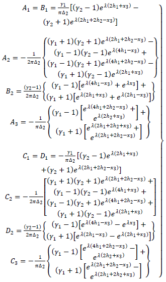
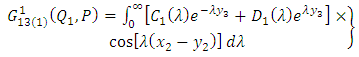
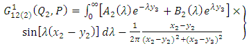
where are the field points in the first layer, second layer and half-space respectively and is any point on the fault F and is the magnitude of discontinuity of across the fault F. According to Rybicki [3], the values of 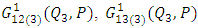are given below

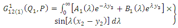(A4)

(A5)

(A6)

(A7)

(A8)

(A9)

where

(A10)

and

(A11)

and

Now

(A12)

First part of (A12)

Now second part of (A12)

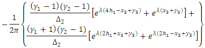Now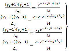

(A13)

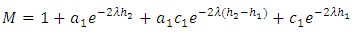Where

where and

Therefore using the result of (A13), we get

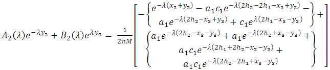(A16)

Now the term (Mondal and Sen [14]) and we can express as an infinite geometric series and neglecting the higher order term and we get from (A16)

Now we assume in the above expressions and putting this value in (A6) and after integration we get

(A17)

Using similar process we obtain that

(A18)

and

(A19)

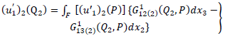
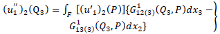
Let is a point on the fault F with respect to the origin O and is any point on F with respect to the origin and a change of co-ordinate system from is connected by the following relations Then on the fault and The discontinuity in is Then from (A1), (A2), (A3) we get

(A20)

(A21)

(A22)

In change co-ordinate system Putting it in (A18), (A17), (A19) and we get the new form of Using these new form of in (A20), (A21), (A22), we get the following results

(A23)

(A24)

(A25)

(A26)

(A27)

(A28)

and

(A29)

(A30)

(A31)

where

(A32)

and

(A33)

(A34)

(A35)

and

(A36)

(A37)

(A38)

(A39)

(A40)

Where

(A41)