Umar Ashraf 1, Peimin Zhu 1, Aqsa Anees 2, Ayesha Abbas 2, Muhammad Afnan Talib 3
1Institute of Geophysics and Geomatics, China University of Geosciences, Wuhan, China
2Faculty of Earth Resources, China University of Geosciences, Wuhan, China
3School of Environmental Sciences, China University of Geosciences, Wuhan, China
Correspondence to: Umar Ashraf , Institute of Geophysics and Geomatics, China University of Geosciences, Wuhan, China.
| Email: |  |
Copyright © 2016 The Author(s). Published by Scientific & Academic Publishing.
This work is licensed under the Creative Commons Attribution International License (CC BY).
http://creativecommons.org/licenses/by/4.0/

Abstract
Balkassar area envelops itself in the Potwar sub basin in Himlayan collisional regime tacitly known for its hydrocarbon structural traps. Proposed research was conducted via SEG Y and well data issued by DGPC using licensed K-tron software. The aftermaths of the research delineate the compressional regime due to thrust faulting. Heretofore, five reflectors were marked based on stratigraphic studies and after correlating with well tops were named as Chorgali, Sakesar, Lockhart, Khewra and Basement. Initially time sections were prepared and were converted to depth section via velocity analysis system to delineate subsurface structure. Fundamental outcome of this research was helpful to velocity factor in affirming the interpretation. It shows the significance of lateral velocity variations in time to depth conversions which is unnoticed by some interpreters by simply averaging the velocity functions into a single function. Confronting this, velocity model was generated using duo interpolation algorithms. The velocity model indicates the importance of lateral velocity variations. Henceforth, the processed velocity models showcase better results for further analysis on structure evaluation and decision making. Effects of velocity in time to depth conversion using layered cake time model was interpreted. Seismic velocities were interpolated and 2D seismic models had been generated through convolution with a klauder wavelet using velocity models. Duo Spatio-temporal and horizon interpolation are best description of velocity modeling and interpolation. Corollary results indicate that horizon based interpolation expatiates best velocity model and thus used in time to depth conversion.
Keywords:
Seismic, Velocity, Stratigraphy, Interpretation, Modeling, Interpolation
Cite this paper: Umar Ashraf , Peimin Zhu , Aqsa Anees , Ayesha Abbas , Muhammad Afnan Talib , Analysis of Balkassar Area Using Velocity Modeling and Interpolation to Affirm Seismic Interpretation, Upper Indus Basin, Geosciences, Vol. 6 No. 3, 2016, pp. 78-91. doi: 10.5923/j.geo.20160603.02.
1. Introduction
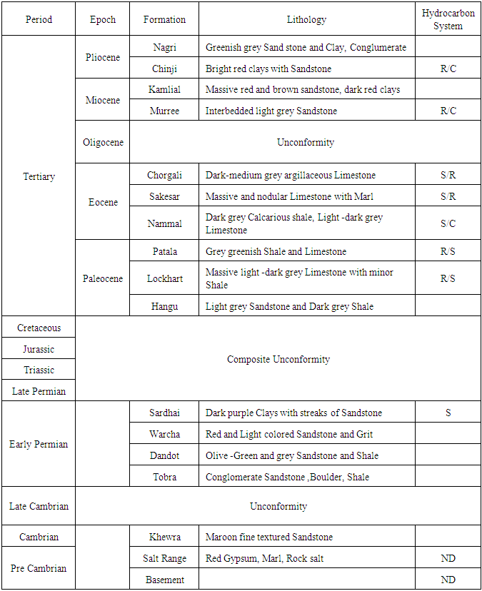
Hydrocarbons are one of the most mandatory constituents while describing the economics of any country. The necessity of delineating those buried hydrocarbons and structures is of extreme importance of geophysical studies. Proposed research of Balkassar area using K-tron software was conducted to reveal the structural information. The Balkassar area is located about 100km southwest of capital Islamabad (Figure 3), in the Chakwal district, Punjab Province. The estimate terrain elevation above sea is 506 meters having Latitude: 32°55'59.99" Longitude: 72°39'0.01. Geographically Balkassar abuts borders with Kalar Khar in South, Chakwal city in East and Talagang city lies towards West. Directorate General Petroleum Concession (DGPC), Government of Pakistan granted the navigation and the velocity data of eleven lines. Base map of the Balkassar area (Figure 1) was generated via K-tron Precision Matrix an Integrated Geo Systems application [1] which lies in Universal Transverse Mercator (UTM, Zone 43) projection system. Proposed study area lies in south eastern part of the Salt Range Potwar foreland basin (SRPFB) bounded by Salt Range thrust in south, Main Boundary thurst (MBT), Kala-Chita and Margalla hills in the north and left lateral Jehlum fault, Jhelum River, Hazara Kashmir Syntaxes in the east and right lateral Kalabagh fault, Indus River, Kohat Plateau is located in the west[2] Potwar sub-basin was originated because of the intense Himalayan collisional orogeny and represents thrust sheets of Precambrian to recent rocks comprised of Northern Potwar Deformed Zone (NPDZ) and Southern Potwar Platform Zone (SPPZ) separated by asymmetrical Soan Syncline. General Stratigraphy of Potwar Basin is given in Table 1.Table 1. Stratigraphic Chart of Area
 |
| |
|
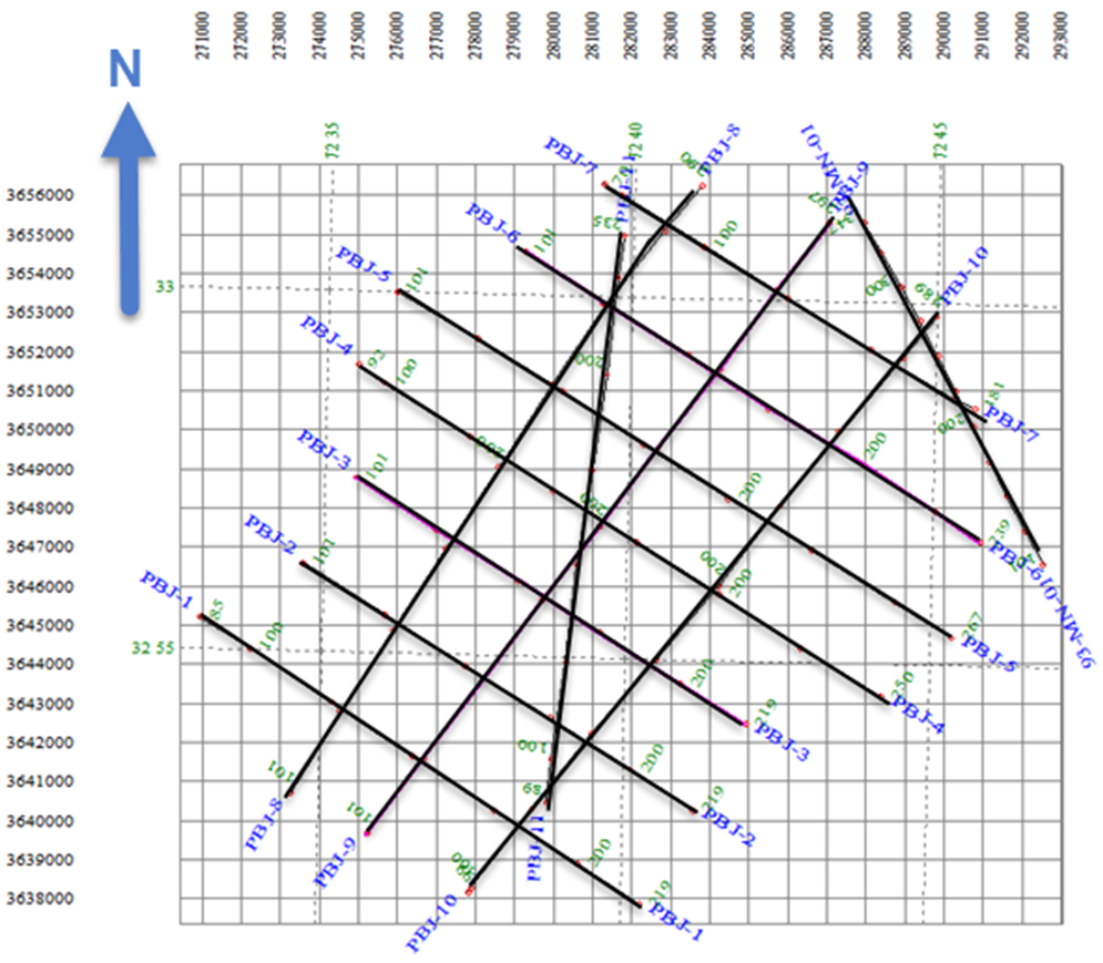 | Figure 1. Base map of the Balkasaar Area displaying seismic lines (Khan, 2000) |
2. Work Flow and Methodology
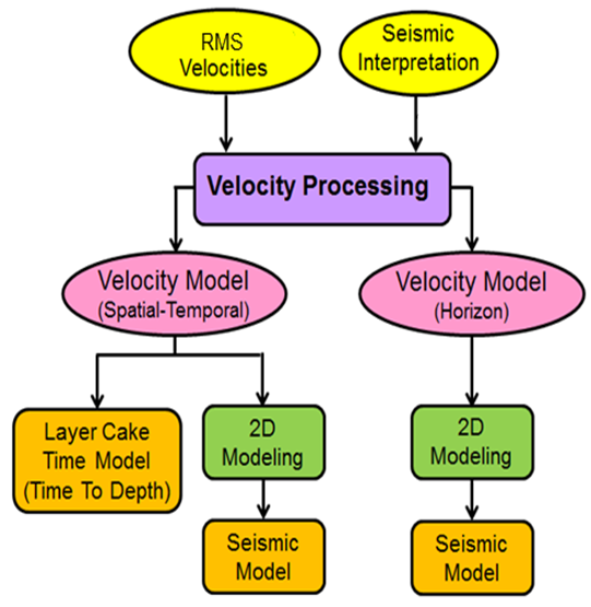
Narrating the workflow and software used (Figure 2), a series of genre modules of Ktron software were accomplished to perform various processes to explain outcomes. The complete work flow showcases the software tools being used along with the processes is given in Figure. Initially reflectors were marked on the basis of prominent reflection on the lines from subsurface interfaces with different colors so that to display the disparity amongst them. Velocities were calibrated using Velocity Analysis System (VAS) [1] and was used in time to depth conversion. Latterly work flow for velocity modeling techniques was accomplished using two interpolation algorithms. Moreover, 2D modeling was performed to confirm structural interpretation. Rock Physics and Engineering Properties for the confirmation of seismic interpretation were also calibrated.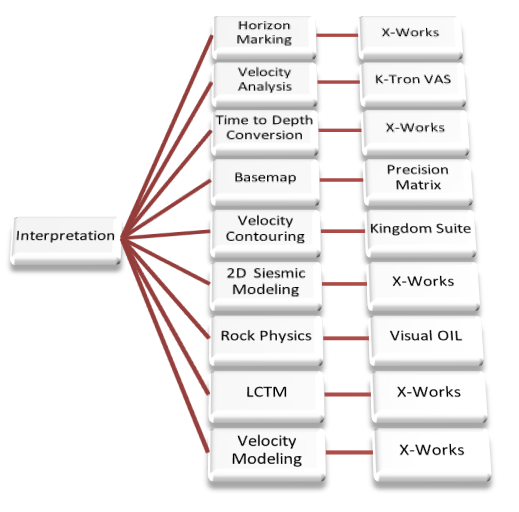 | Figure 2. Interpretation Work and the software modules used for Research |
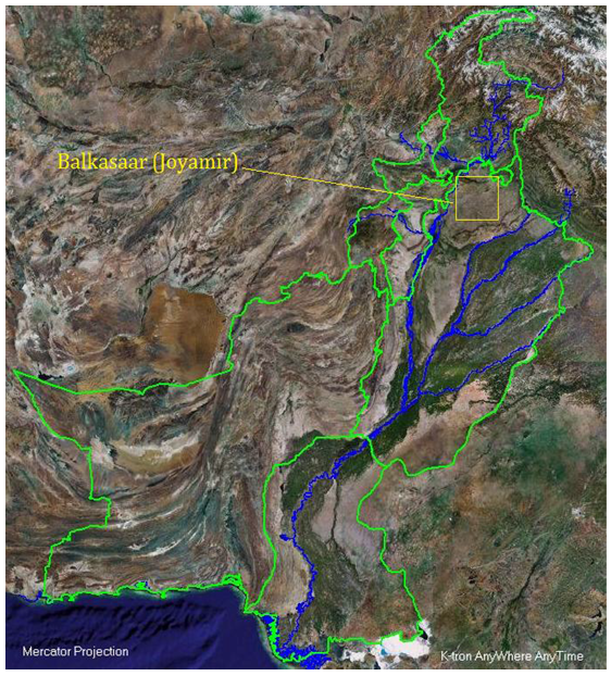 | Figure 3. Satellite image of Pakistan showing Balkassar area [5] |
 | Figure 4. Velocity modeling techniques and their applications |
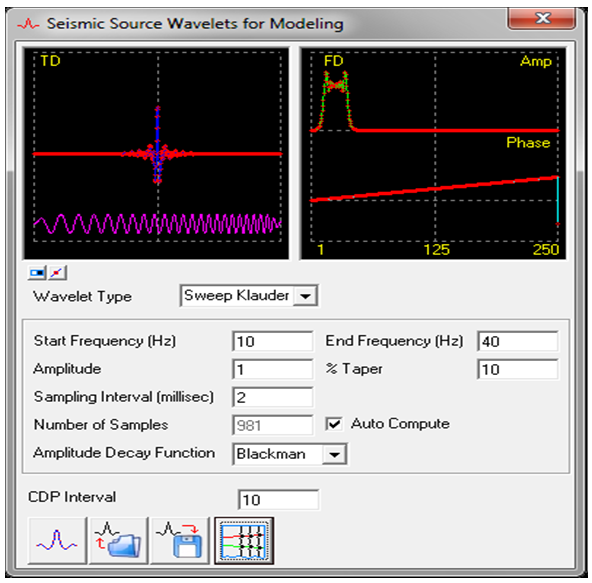 | Figure 5. A Sweep Klauder wavelet Generated with frequency 10-40 Hz with 10 % tapering and Blackman Amplitude Decay Function as a source for 2D Seismic Modeling |
3. Results and Discussions
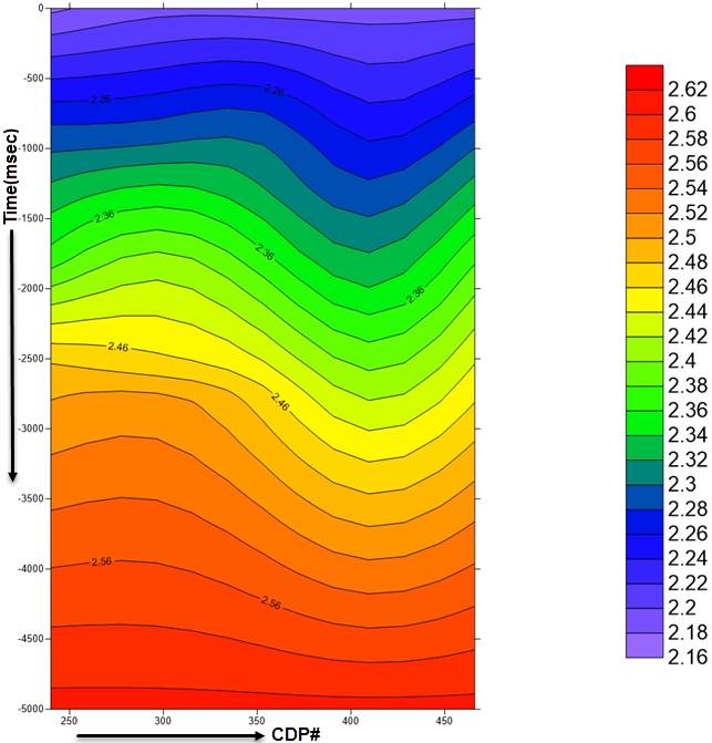
Seismic InterpretationOn seismic lines, reflectors were identified on the basis of prominent adjacency of reflectors from the subsurface interfaces. Each reflector was marked with different color as to disseminate the disparity amongst them. Moreover, secondary information of subsurface depths was utilized from well data to pick five prominent reflectors. The Chorgali formation which is limestone reservoir displays prominent reflections on seismic section. The radical reflectors marked on the seismic sections that are of interest are Chorgali, Sakesar, lockhart and khewra formations. Categorically the time section annotates the position and configuration of reflectors in time domain. Reflectors were marked on seismic line PBJ-05 and named explicitly on the basis of stratigraphic column encountered in well Balkassar Oxy -01. However, the attempt is to investigate the source, reservoir and seal rock formations. Ingenuously seismic image is inadequate for an exploration or field development interpretation. Appropriate well ties and reliable depth conversion are also important. The seismic sections are in time domain (Figure 6) and are insufficient to delineate the results, as the subsurface structures are in depth domain so time sections were modified to depth sections using velocities data. X-Works reads velocity data in IGS Velocity format for time to depth conversion. The seismic section velocities are Root Mean Square (RMS) velocities. These must be converted into interval and finally average velocities for time to depth conversion. The seismic velocities are processed (Converted, Interpolated and Smoothed) by using Velocity Analysis System (VAS) [3] (Figure 7) used for Time-to-Depth conversion and Modeling. The velocity data is converted into the X-Works format using data formatting scripts available in Visual OIL. The input seismic velocities (Root Mean Square) in IGS velocity format are uploaded in X-Works and a spatio-temporal or horizon Interpolated velocity model is generated. Lateral and vertical velocity variations provide true depth imaging using velocity model. The horizon velocity map of Chorgali is shown. (Figure 8). These velocities were multiplied with time of each reflector and divided by two to acquire the depth section (Figure 9).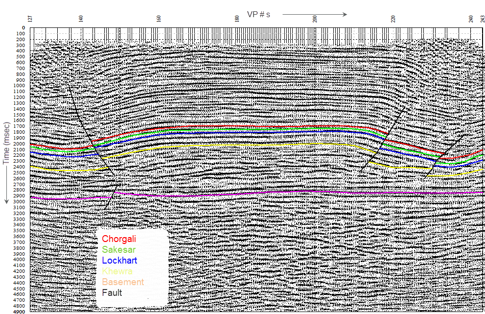 | Figure 6. Interpreted Time Section of Seismic Line PBJ-05 (Chorgali: Red, Sakesar: Green, Lockhart: Blue, Khewra: Yellow Basement: Pink) |
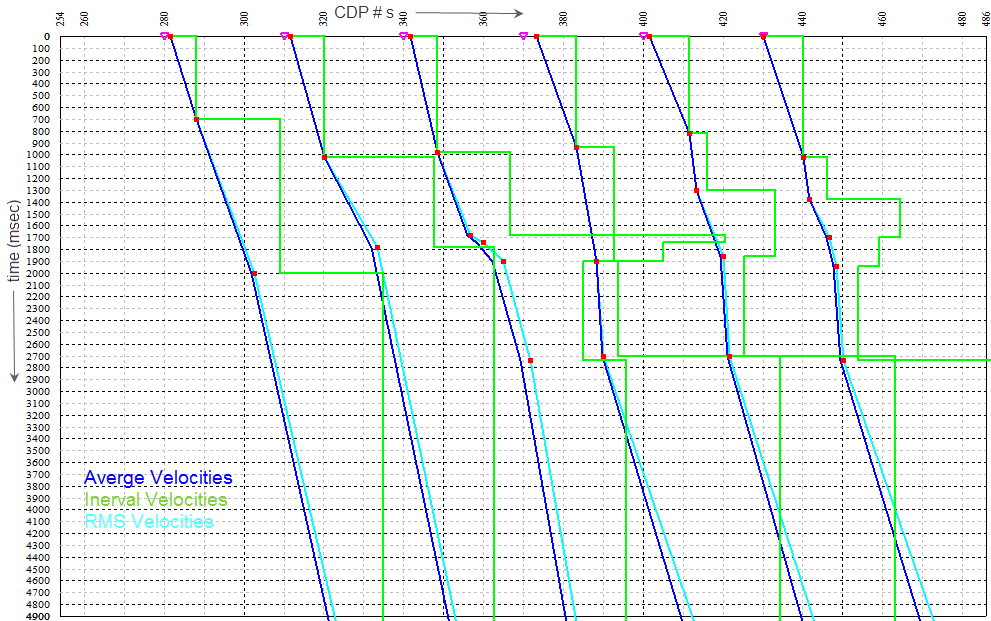 | Figure 7. Seismic velocities of line PBJ-05 combine displayed at different CDPs |
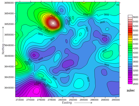 | Figure 8. Horizon Velocity Contour Map of Chorgali Formation |
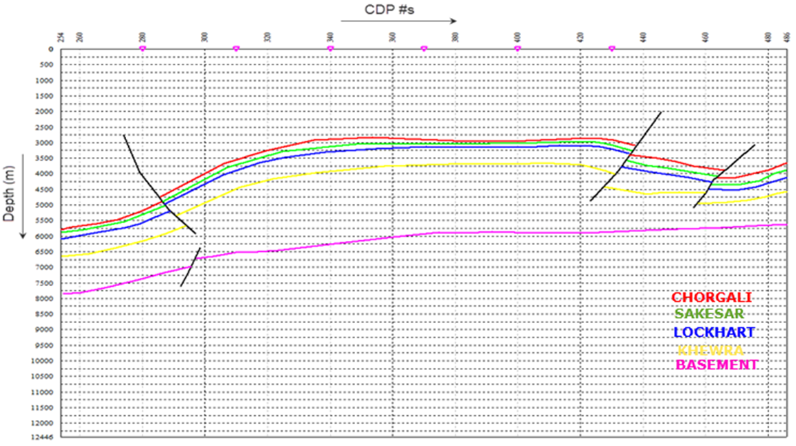 | Figure 9. Depth Section of seismic line PBJ-05 |
Volume of shaleOxy-01 depicts reservoir and source zones. The shale signature is prominent in the areas closely matching the location of Patala and Dhandot at depth 2600 and 2850 as given by the information from the well tops, while the zones located above the shale signature indicates the reservoir zone at the depth of 2400-2600 meters which is approx. depth of Chorgali and Sakesar formation. The Gamma Ray log along with sand and shale lines are linearly computed. (Figure 10)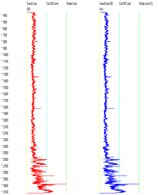 | Figure 10. Gamma Ray log (Red) along with calculated Volume of Shale curve (Blue). [Sky-Blue=cutoff line, Green=shale line and Yellow=sand line] |
Rock PhysicsTo compute the rock physical and engineering properties, velocity functions were used. Interval velocities are used, which represent the true lithological properties of the sub-surface layers. The velocity functions are processed to compute rock physics sections using a scripted program written in Visual OIL [4]. Cross-sections of rock properties such as density (Figure 12) and porosity (Figure 11) have been generated to understand the variation of these parameters across the sections.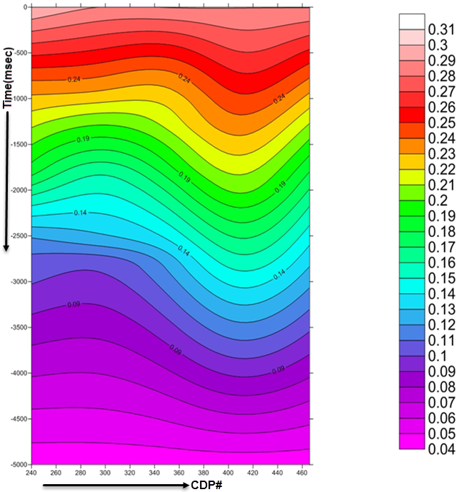 | Figure 11. Porosity Cross-Section of line PBJ -06 |
 | Figure 12. Density section showing the variation of Density along the seismic line PBJ-06 |
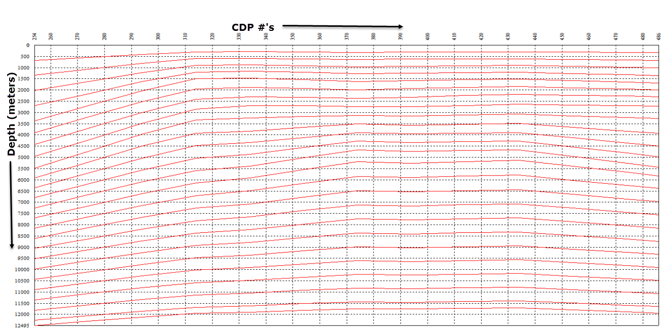
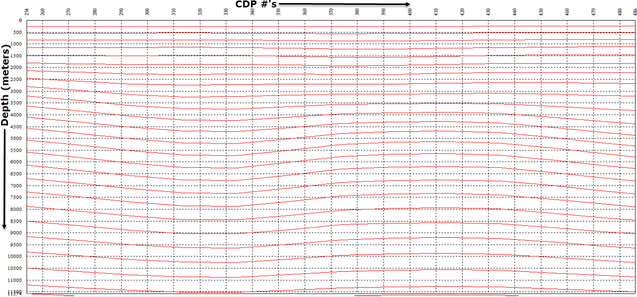
Spatio-Temporal Velocity InterpolationThe X-Works provide us with the Spatio-Temporal Velocity Interpolation Feature. The RMS velocity functions are basically velocity-time pairs (VT-Pairs) without fixed time intervals. In this technique, first temporal (vertical) interpolation of 100 milliseconds is applied to get velocity functions with VT-Pairs after regular time intervals. If required, then 3 to 5 point moving average operator is applied along each function to get vertical smoothing of velocities. Next spatial interpolation at 5th CDP is applied to generate velocity functions at the specified CDP interval. This is followed by a 3 to 5 point moving average operator across the velocity functions or along the time slice to get lateral smoothing of velocities. This generates the spatio-temporal interpolated RMS velocity model. (Figure 13)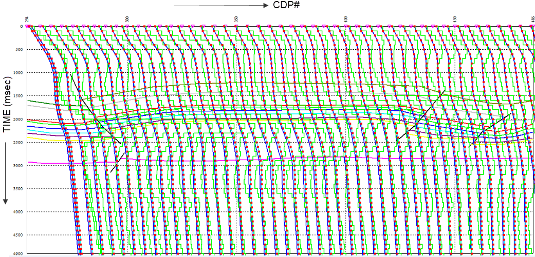 | Figure 13. Spatio-temporal Velocity model using spatial interpolation at 5 CDP intervals RMS velocities (Light-Blue) Interval (Dark Green) Average (Dark Blue) velocities |
Horizon Velocity InterpolationHorizon interpolation is composite interpolation method which requires input of interpreted horizons, in addition to the velocity data. The velocity was interpolated along these horizons, instead of interpolation along the time slice (Figure 14). It requires computation of nodes for each horizon at the specified CDP interval. VT-Pairs are then interpolated at these nodes to generate velocity functions. The velocity model generated by this technique closely matches the subsurface as structures as shown in Figure. Compendiously these sorts of velocity models are commonly used for velocity imaging using modeling and Pre-Stack Depth Migration (PSDM).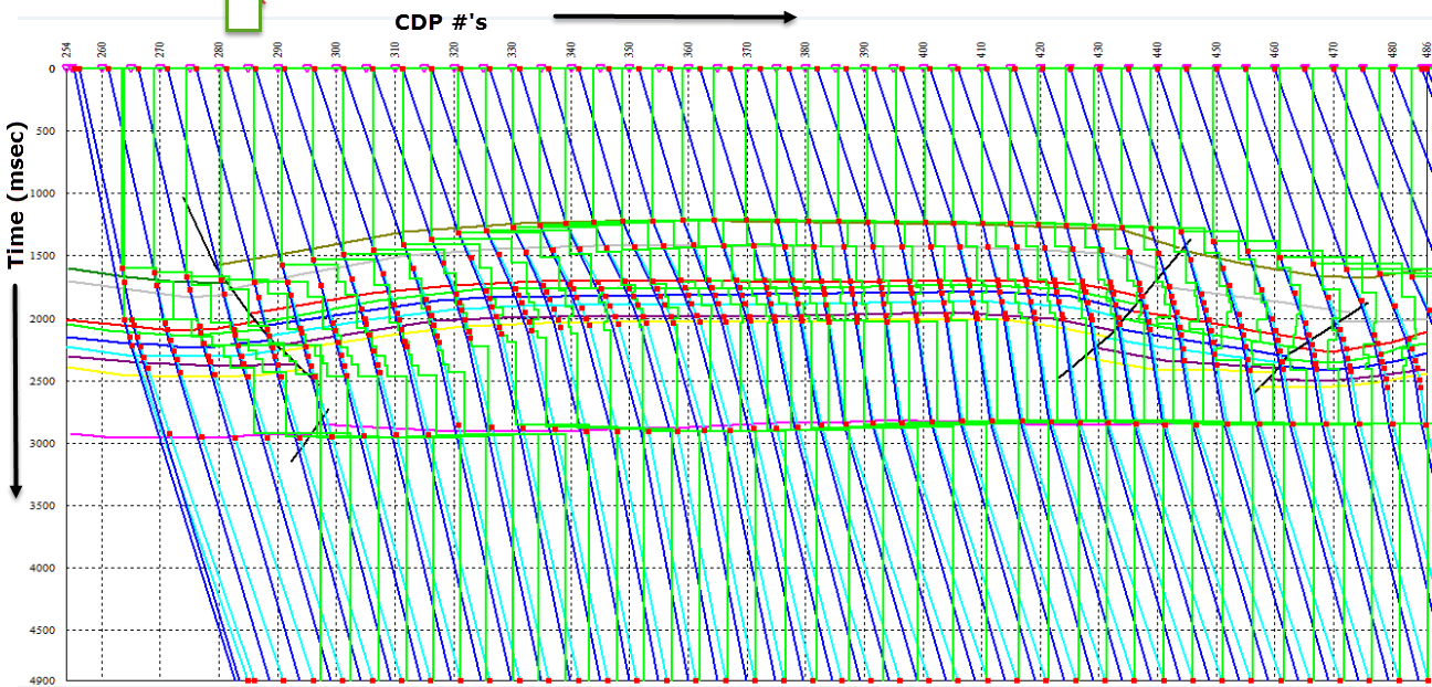 | Figure 14. Velocity model generated by interpolation of velocity functions at every 5th CDP along the interpreted horizons RMS velocities (Light-Blue) Interval (Dark Green) Average (Dark Blue) velocities |
LCTMA Layered Cake Time Model (LCTM) consisting of flat horizons or time slices after every 100 milliseconds with nodes at every 5th CDP was generated for PBJ-05 seismic line (Figure 15). The calibrated velocity functions are loaded and processed to generate an unsmoothed spatio-temporal velocity model with a temporal interval of 50 milliseconds and spatial interval of 5 CDP as narrated earlier. Velocity model was then used in time to depth conversion of the LCTM to generate a depth section (Figure 16) which depicts the deformation of the LCTM in the form of pull ups & downs in the depth section due to lateral velocity variations. Tacitly the attained depth section is not smooth due to fluctuations in the velocity model. Thus a spatio-temporal smoothing with a 3x3 kernel operator is applied to generate a smoothed velocity model, which is again used in time to depth conversion of LCTM. The resulting depth section was much smoother as compared to that (Figure 17). Corollary, it concludes that velocity models must be smoothed to get realistic time to depth conversions. It also shows the significance of lateral velocity variations in time to depth conversions which is unnoticed by some interpreters by simply averaging the velocity functions into a single function.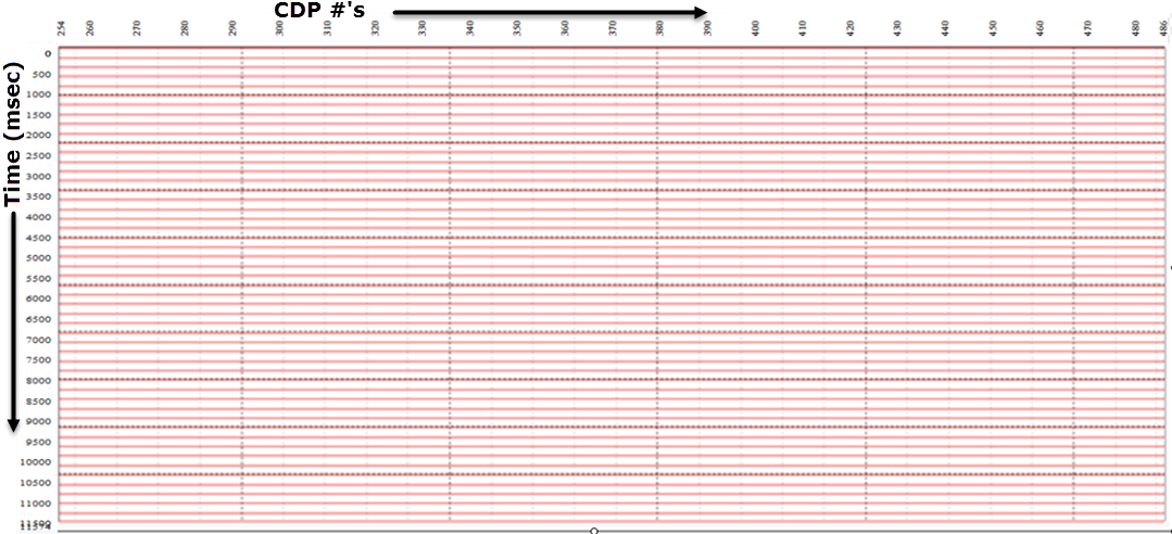 | Figure 15. Layered Cake Time Model (LCTM) of seismic line PBJ-05 |
 | Figure 16. Depth converted LCTM with sharp pull ups and pull downs due to lateral velocity variations |
 | Figure 17. Effect of smoothed velocities on a depth converted section |
2D Seismic Modeling based on velocity functions2D seismic models were generated for line PBJ-05 using three methods. First two were generated from the velocity models explained earlier, while the third is generated from the interpreted seismic depth sections. In all these methods a klauder wavelet of 10-80 Hz sweep frequencies with 20% linear tapering with a blackman amplitude decaying function was used as a source (Figure 5). The wavelet was convolved with velocity models or interpreted depth section at every 10 CDP to generate a seismic section. As the modeling is applied at zero offset, the resulting synthetic seismic model is a migrated section. The three seismic modeling techniques are discussed below.2D Seismic Modeling based on Spatio-Temporal Velocity interpolationThe spatio-temporal interpolated velocity model was used as input. The RMS velocity functions are converted into interval velocity functions. The VT-pairs in these functions were at regular intervals and therefore they do not portray the sub-surface structural information. The interval velocity functions were used to generate reflectivity series which in turn are convolved with the source wavelet to generate seismic traces forming a 2D seismic model (Figure 18). It can be considered that the seismic section generated from this method does not show any structural features. Corollary it concludes that structural information contained in original velocity functions is lost due to spatio-temporal interpolation. Thus spatio-temporal interpolated velocity models can be used in time to depth conversion, but they cannot be used in modeling and rock physics applications.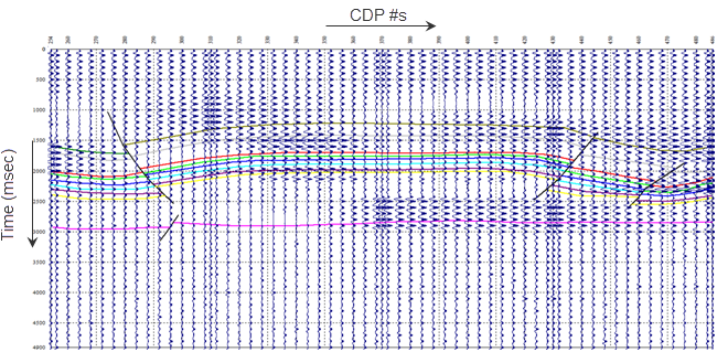 | Figure 18. 2D seismic model generated by using spatio-temporal velocity interpolated model without seismic |
2D Seismic Modeling based on Horizon Velocity interpolationThe basic modeling procedure is the same as elaborated earlier, except horizon interpolated velocity model is used as input. The model seismic section generated by this technique is shown in Figure 4. It can be observed that this seismic model displays a reasonable sub-surface image clearly depicting structures whilst zoomed image of 2D seismic model generated by using horizon velocity interpolated model along with seismic is also enclosed (Figure 19).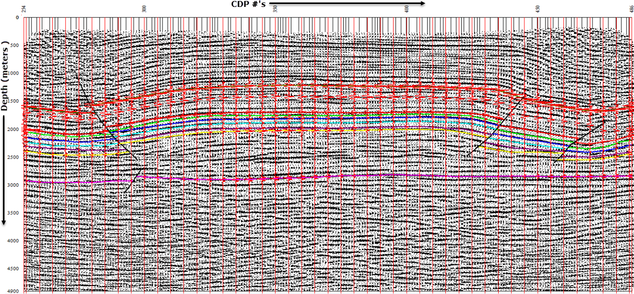 | Figure 19. 2D seismic model generated by using horizon velocity interpolated model with seismic |
Seismic Model based on 2D Interpreted Depth SectionsThis is the conventional modeling in which the interpreted time section is converted into a depth section. Reflection coefficients are assigned to each reflector as an attribute. The section is convolved with the source wavelet to generate a 2D synthetic seismic section (Figure 20). As this modeling is completely based on the structural data so the derived synthetic section completely matches the structures. This type of modeling is commonly used to adjust acquisition parameters for neo surveys based on geological cross-sections with velocities assigned to each formation and get seismic response of stratigraphic models as well as confirmation of seismic interpretation.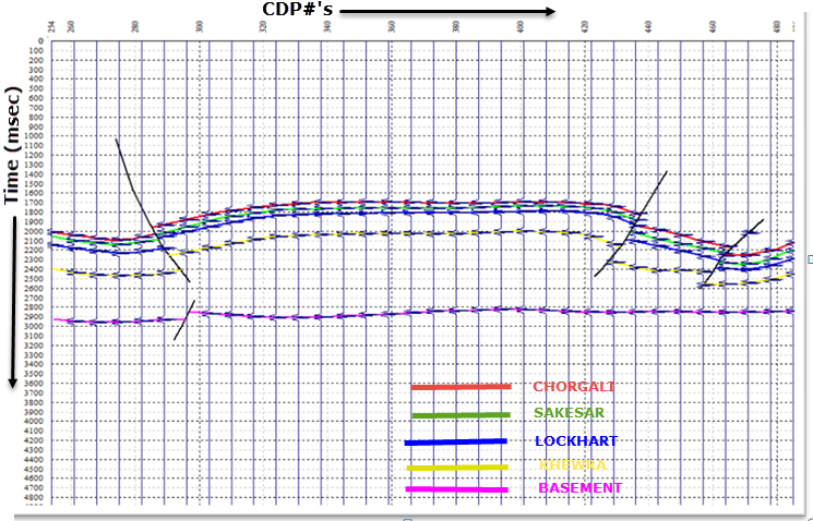 | Figure 20. Synthetic Seismic Section using K-Tron X-Works |
4. Conclusions
ο Interpretation of seismic structural model shows severe thrust faults which confirm the compressional tectonic regime with anticlinal structure in the proposed area.ο Rock properties are calculated, these are helpful to confirm the nature and type of sub-surface material. Porosity and density are used to confirm the reservoir.ο The Iso-velocity contour map shows the vertical and lateral variation in velocity due to compaction of material with the depth of burial as well as lithological changes (both vertically and laterally).ο Velocities vary latterly as well as vertically. Due to various types of velocities and diverse parameters and usages, this fact must be taken into consideration during processing and interpolation of velocity data. While appropriate smoothening must be applied to acquire true depth sections.ο Spatio-temporal velocity model with smoothening operators are satisfied and are recommended for time to depth conversion. Unfortunately, this model cannot be used for modeling applications as the structural information is obscure during time-slice interpolation.ο Horizon interpolated velocity model is vigilant and reliable but its algorithm is very complex. Availability of productive computing power with appropriate software tools, this model can now be studied adeptly and is recommended for time to depth conversions, seismic modeling and Pre-Stack Depth Migration (PSDM).
5. Recommendations
ο Seismic data affirms interpretation as the usage seismic data is of ultimate necessity.ο Velocity modeling based upon interpolation shouldn’t be neglected because it illustrates the lateral and vertical variations.ο Horizon based velocity interpolation is most productive and must be used as it displays correct results for the time to depth conversion.
ACKNOWLEDGMENTS
I am thankful to DGPC to give me with the seismic data and to Sir Khalid Amin Khan (OIST) for his moral and technical manner which was quite helpful and I found it quite satisfied amending my knowledge regarding seismic under his supervision.
References
| [1] | Khan, K.A., Computer Applications in Geology, No. 4, Chapter 16: Integrated Geo-Systems -- A Computational Environment for Integrated Management, Analysis, and Presentation of Petroleum Industry Data. 2000. |
| [2] | Kazmi, A.H. and M.Q. Jan, Geology and tectonics of Pakistan. 1997: Graphic publishers. |
| [3] | Khan, K. A. and G. Akhter, Work flow shown to develop useful seismic velocity models. Oil and Gas Journal, 2011. 109(16): p. 52-61. |
| [4] | Khan, K.A., G. Akhter, and Z. Ahmad, OIL—output input language for data connectivity between geoscientific software applications. Computers & Geosciences, 2010. 36(5): p. 687-697. |
| [5] | Khan, K.A., et al. Development of a projection independent multi-resolution imagery tiles architecture for compiling an image database of Pakistan. in Advances in Space Technologies, 2008. ICAST 2008. 2nd International Conference on. 2008. IEEE. |

 Abstract
 Reference
 Full-Text PDF
 Full-text HTML