-
Paper Information
- Paper Submission
-
Journal Information
- About This Journal
- Editorial Board
- Current Issue
- Archive
- Author Guidelines
- Contact Us
Geosciences
p-ISSN: 2163-1697 e-ISSN: 2163-1719
2016; 6(2): 29-40
doi:10.5923/j.geo.20160602.01

Long Vertical Strike-Slip Fault in a Multi-Layered Elastic Media
 Abstract
 Reference
 Full-Text PDF
 Full-text HTML
1Joka Bratachari Vidyasram Girls’ High School, India
2Department of Applied Mathematics, University of Calcutta, India
Correspondence to: Bula Mondal, Joka Bratachari Vidyasram Girls’ High School, India.
| Email: |  |
Copyright © 2016 Scientific & Academic Publishing. All Rights Reserved.
This work is licensed under the Creative Commons Attribution International License (CC BY).
http://creativecommons.org/licenses/by/4.0/

The lithosphere-asthenosphere system has been represented by a multi-layered model consisting of two elastic layers overlying an elastic half-space. A vertical buried strike-slip fault is taken to be situated in the uppermost layer. The fault undergoes a sudden slip under the action of tectonic forces due to mantle convection. Analytical expressions for displacements, stresses and strains are obtained both before and after the fault movement for both elastic layers as well as the elastic half-space. It has been observed that due to the fault movement there are regions where stresses accumulate, and there are other regions where stresses reduce. The contour map for the stress-pattern in the first layer has been prepared.
Keywords: Lithosphere-asthenosphere system, Aseismic state, Strike-slip fault, Mantle convection, Sudden movement
Cite this paper: Bula Mondal, Sanjay Sen, Long Vertical Strike-Slip Fault in a Multi-Layered Elastic Media, Geosciences, Vol. 6 No. 2, 2016, pp. 29-40. doi: 10.5923/j.geo.20160602.01.
Article Outline
1. Introduction
- Occurrence of earthquake is usually a cyclic phenomena. About 90% of all earthquakes are natural which are the results of tectonic events primarily due to movement across the faults. Two major seismic events are separated by a long asesimic period in seismically active region. For better understanding of the earthquake processes it is necessary to study the stress accumulation pattern in the region during the aseismic period. Such studies can be done by developing suitable theoretical models with the essential features of the local geological structure and the earthquake faults situated in the lithosphere-asthenosphere system. The lithosphere-asthenosphere system may be represented by a multi-layered half-space model due to many inhomogeneities in it with respect to elastic properties. Many authors such as Maruyama [1], Rybicki [2, 3], Mukhopadhyay [4, 5], Debnath and Sen [6-9], Debnath and Sen [10-12] represented the lithosphere-asthenosphere system either by an elastic/ viscoelastic half-space or by a layered viscoelastic half-space. In our model we however consider a multi-layered elastic medium consisting of two elastic layers of finite depth overlying an elastic half-space to represent the lithosphere-asthenosphere system.
2. Formulation
- We consider a theoretical model of lithosphere-asthenosphere system as three-layered elastic half-space with different rigidities. It is assumed that the medium is made up of two parallel, isotropic and homogeneous elastic layers lying over an isotropic homogeneous elastic half-space. The layers and half-space are in welded contact. The depth of the boundary dividing two elastic layers from free surface is
 and the depth of the boundary dividing second elastic layer and elastic half-space is
  . A buried vertical strike-slip fault whose length is large compared to its width l is taken to be situated in the first layer. The depth of upper edge of the fault below free surface is
  and the upper and lower edges of the fault are horizontal. We now introduce a rectangular Cartesian co-ordinate system
  with the plane free surface as the plane
  is pointing downwards into the medium and
  is taken along the upper edge of the fault on the free surface.
  and
and  give the boundary surfaces between two layers and second layer and half-space respectively. For convenient of analysis we introduce another set of Cartesian co-ordinate system
  with the upper edge of the fault as
  and the plane of the fault as the plane
  , so that the fault F is given by
  . The relations between two co-ordinate systems are given by
  | (1) |
 , the second elastic layer occupies the region
 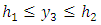 and the elastic half-space occupies the region
  . The Figure 1 shows the section of the theoretical model by the plane
  .
. | Figure 1. Section of the model by the plane y1 = 0 |
 and are functions of
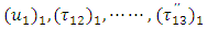
  . Then the components of displacement, stress and strain will separated out into two distinct and independent groups, one associated with strike-slip movement and other associated with dip-slip movement of the fault. The components of displacements, stresses and strains associated with strike-slip movement of the fault are
  for first elastic layer,
  for second elastic layer and
  for elastic half-space respectively.
2.1. Stress-Strain Relations
- The constitutive equations for the first elastic layer
 are taken as:
  | (2) |
 are
are 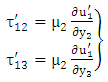 | (3) |
 are
are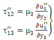 | (4) |
 are rigidities of two layers and half-space respectively.
2.2. Stress Equation of Motion
- For a slow, aseismic, quasi-static deformation of the system, the inertial terms in the stress equation of motion are very small and can be neglected as explained by Mukhopadhyay et. al. [13]. Then stress equation becomes
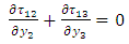 | (5) |
 | (6) |
 | (7) |
 .From equation (2)-(7) we get
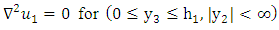 | (8) |
 | (9) |
 | (10) |
2.3. Boundary Conditions
- We measure the time t from a suitable instant when the model is in aseismic state and there is no seismic disturbance in it. Since the free surface is stress free and the two layers and second layer and half-space are assumed to be in welded contact, then the boundary conditions are
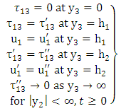 | (11) |
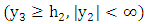
2.4. Conditions at Infinity and Initial Conditions
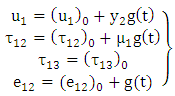
 are the values of
  at time t = 0 and they satisfy all the relations stated above. We assume that, at a large distance from fault plane there is a shear strain maintained by some tectonics forces (Kasahara [14]), such as mantle convection (Fowler [15]), etc. and then we have the following conditions
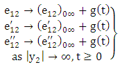 | (12) |
 ,
,  ,
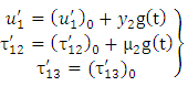
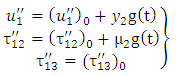
,  , where
  are the values of
  at t = 0 and g(t) is a slowly increasing, continuous function of t with g(0) = 0. Same g(t) is taken for layers and half-space, since they are in welded contact, so that strains are continuous at the boundaries.
3. Displacements, Stresses and Strains in the Absence of Fault Movement
- In this case the displacements, stresses and strains are continuous throughout the system. To obtain the solutions in the absence of fault movement we solve the boundary value problem given by (2)-(12) and get the solution in the following form
 | (13) |
 | (14) |
 | (15) |
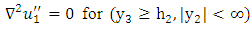
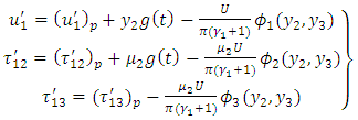
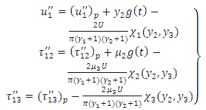
4. Displacements, Stresses and Strains after Restoration of Aseismic State after a Sudden Movement across the Fault
- It is to be noted that due to the sudden fault movement across the fault F, the accumulated stress will be released at least to some extent and the fault becomes locked again. For a comparatively short period of time during and after sudden fault movement when the seismic disturbances are present, inertial terms are not small and cannot be neglected. So we leave out this short period of time and consider the model after restoration of aseismic state. From this state we measure the time t afresh. In this second phase of aseismic state the equations (2)-(10), boundary conditions (11), (12) and initial conditions are valid.The displacements, stresses and strains are continuous everywhere in the model except on the fault F across which the displacement component
 has a discontinuity which characterizes the sudden movement across the fault F. The discontinuity of
  across F is defined as
 | (16) |
 and
and  is a continuous function of
  and U is constant, independent of
  . All the other components
  are continuous everywhere in the model.To solve the above boundary value problem with new time origin
  for displacements, stresses and strains during aseismic state after commencement of sudden fault movement, we try to find the solutions in the following form
 | (17) |
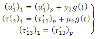
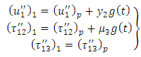
 represent the effect of displacements, stresses and strains present at t=0 and satisfy all the equations (2)-(12) and continuous throughout the medium while
 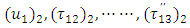 represent the effect of sudden fault movement across F and satisfy all the above relations (2)-(11) and also satisfy the dislocation condition (16) together with
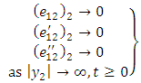 | (18) |
 | (19) |
 | (20) |
 | (21) |
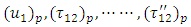 are the values of
 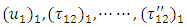 respectively at t=0 (i.e. new time origin).Now to solve the boundary value problem containing
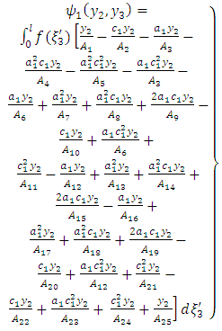
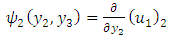
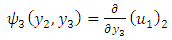
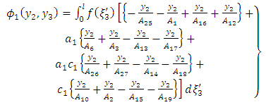
  we use Green’s function technique developed by Maruyama [1] and Rybicki [2, 3] as explained in Appendix. The required solutions are obtained as
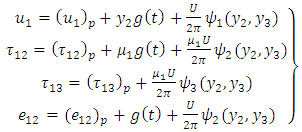 | (22) |
 | (23) |
 | (24) |
 and analytical form of
  are given in Appendix.It is found that the displacements, stresses and strains will be finite and single valued anywhere in the model if the following conditions are satisfied(i)
  and
and  are both continuous functions of
  for
for  .(ii) f(0) = 0, f(l) = 0 and
  (iii) Either
  is continuous in
  is continuous
  except for a finite number of points of finite discontinuity in
  is continuous in
  except possibly for a finite number of points of finite discontinuity and for the end points of [0, l], there exist real constant m, n both < 1 such that
  or a finite limit as
  and
and  or to a finite limit
  .
.5. Numerical Computations
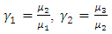
- It is assumed that due to some tectonic reason there is a slow but steady accumulation of shear strain at a distance far away from the fault. Keeping this in view we take g(t) to be linearly increasing with time and g(0) = 0. With this assumption, we take g(t) = kt. From major earthquakes it has been observed that the stress release may be of the order of 400 bars. So we assume
 , noting also that the observed rate of strain accumulation in seismically active regions during the aseismic period is of the order of 10-6 to 10-8 per year. For
  and
and  the rigidities of the layers and half-space, We take
  ,
,  ,
,  as suggested by Aki [16], Bullen [17], Cathles [18], Chift [19], Karato [20] for lithosphere-asthenosphere. For
  the thickness of the layers we take
  depth of upper edge of the fault below free surface = 5 km. For l, the width of the fault, we use l = 10 km. noting that for San Andreas fault in North America, the value of l has been estimated to be in the range 5-15 kms. U = 40 cm corresponding to the observed relative displacements on the surface for moderate buried strike-slip fault movement. We take
  which satisfies the conditions as stated earlier for bounded stresses and strains everywhere in the model.We now compute the following quantities:(i)
  The residual/ additional surface shear strain due to fault movement near the fault after restoration of aseismic state
  (ii)
(ii)  Change in shear stress in first layer due to fault movement after restoration of aseismic state.
 The Figure 2 shows that the change of the residual/ additional surface shear strain with distance
  from the fault. The fault movement leads to release of the surface shear strain near the fault and the effect is symmetrical about the fault trace. The magnitude of the surface shear strain release due to fault movement is maximum near the fault trace and this strain release falls off rapidly as we move away from the fault on the surface and becomes very small for large values of
  . The magnitude of surface shear strain accumulation is found to be of the order of
  which is in conformity with the observed ground deformation during aseismic period in seismically active regions.
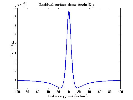 | Figure 2. Additional surface shear strain due to fault movement |
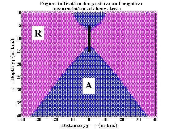 | Figure 3. Region indication for positive and negative accumulation of shear stress |
 with the depth
  for different values of
  . Here, for the first layer the region bounded by the upper and lower edges of
  , the shear stress
  is found to release in general irrespective of the distance
  from the strike of the fault. The magnitude of reduction is higher for point nearer to the fault. For
  gradually tend to zero.
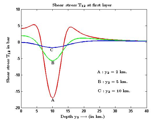 | Figure 4. Comparison of shear stress at different y2 in the first layer |
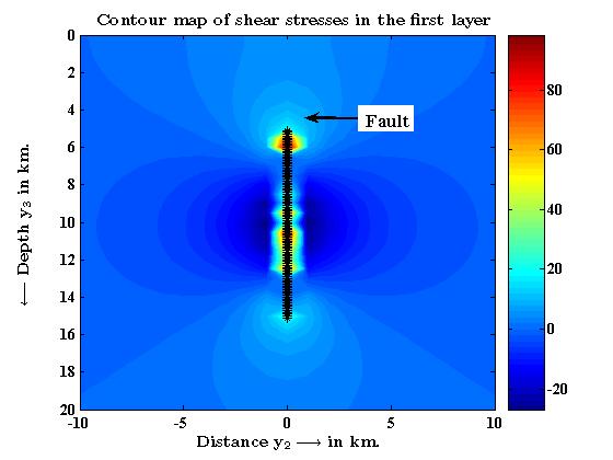 | Figure 5. Contour map of shear stresses in the first layer |
6. Conclusions
- It is observed that there are certain regions of stress accumulation in the first layer and certain other regions of stress release. The rate of stress accumulation/ release in the layer near the fault may be used to compute the happening of the next major event.
ACKNOWLEDGEMENTS
- One of the authors Bula Mondal thanks the Head Mistress of Joka Bratachari Vidyasram Girls’ High School for allowing me to pursue the research, and also thanks the Geological Survey of India; Department of Applied Mathematics, University of Calcutta for providing the library facilities.
Appendix
- Solutions of displacements, stress and strain in aseismic state after sudden movement across the fault:The displacements, stress and strains for
 with new time origin after restoration of aseismic state followed by a sudden movement have been found in the form given by (17) where
  are given by (19)-(21) and
  satisfy (4.2)-(4.11), (16) and (18).This boundary value problem involving
  can be solved by using modified Green’s function technique developed by Maruyama [1] and Rybicki [3]. According to them,
 | (A1) |
 | (A2) |
 | (A3) |
 are the field points in the first layer, second layer and half-space respectively and
  is any point on the fault F and
  is the magnitude of discontinuity of
  across the fault F. According to Rybicki [3], the values of
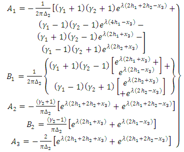
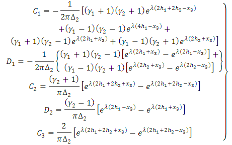
  are given below
 | (A4) |
 | (A5) |
 | (A6) |
 | (A7) |
 | (A8) |
 | (A9) |
 | (A10) |
 and
and  | (A11) |
 Let
Let  is a point on the fault F with respect to the origin O and
  is any point on F with respect to the origin
  and a change of co-ordinate system from
  to
to  is connected by the following relations
  ,
,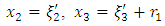 . Then on the fault F,
  and
and  . The discontinuity in
  is
is  . Then from (A1), (A2), (A3) we get
 | (A12) |
 | (A13) |
 | (A14) |
 | (A15) |
 Now
Now Now second part of (A15)
 where
where  and
and  . Putting the above values in (A15) we get,
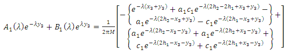 | (A16) |
 Let
Let 
 From Bullen and Bolt [21], we find that
  ,
,  ,
,  . Then
  . Now,
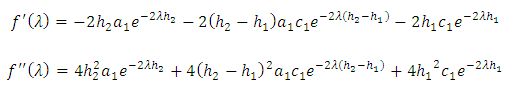
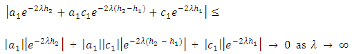 So,
So,  as
as  and
and  and also
  .Hence the function
  is monotonically decreasing. Since
  and
and  is monotonically decreasing, then
  for all values of
  . Therefore,
  for our model. So, we can expand M as an infinite geometric series and neglecting the higher order terms and from (A16) we get
 Now we assume
  in the above expressions and putting this value in (A4) and after integration we get
 | (A17) |
 | (A18) |
 | (A19) |
 . Putting it in (A17), (A18), (A19) and we get the new form of
  . Using these new form of
  in (A12), (A13), (A14), we get the following results
 | (A20) |
 | (A21) |
 | (A22) |
 | (A23) |
 | (A24) |
 | (A25) |
 | (A26) |
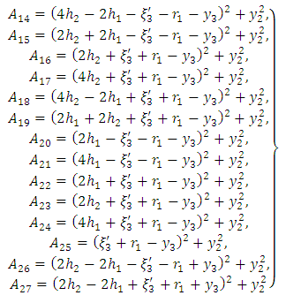
 | (A27) |
 | (A28) |
 | (A29) |
 | (A30) |
 | (A31) |
 | (A32) |
 | (A33) |
 | (A34) |
 | (A35) |
 | (A36) |
 | (A37) |
 | (A38) |