Abderrahim Moujane1, Soumia Mordane2
1Direction de la Météorologie Nationale, Aéroport Casa-Anfa, B.P. 8106 Oasis, Casablanca, Maroc
2Université Hassan II – Mohammedia, Faculté des Sciences Ben M’Sik, Casablanca, Maroc
Correspondence to: Abderrahim Moujane, Direction de la Météorologie Nationale, Aéroport Casa-Anfa, B.P. 8106 Oasis, Casablanca, Maroc.
| Email: |  |
Copyright © 2014 Scientific & Academic Publishing. All Rights Reserved.
Abstract
Moroccan upwelling is the central part of the Canaries system. Along the Canary Current, Major upwelling zones are located in a zone of transition from classical coastal upwelling regions or at the offshore and the immediate coastal area wide of 20 miles. This region lies between Cap Sim and Cap Blanc, where the upwelling persists during the whole year. This geographic zone of Moroccan coasts is characterized by major fishing areas and a high level of oceanographic variability of meso-scale resulting from its geographical heterogeneity. Variations of the continental shelf, the presence of caps and disruption represented by the Canary Islands and headlands produce extended filaments; significant upwelling variability and eddies induced between the islands. This study illustrates the spatial variability of the temperature of the sea surface over the entire area, with a maximum deviation of 0.51°C for measurements and 0.47°C to 0.52°C for simulations.
Keywords:
Upwelling, ROMS, ALADIN, QuiKSCAT, Forcing
Cite this paper: Abderrahim Moujane, Soumia Mordane, The Seasonal and Interannual Variability of Moroccan Upwelling, Geosciences, Vol. 4 No. 2, 2014, pp. 42-50. doi: 10.5923/j.geo.20140402.03.
1. Introduction
The study of upwelling system has known great improvements with the event of remote sensing. It is possible now to study the relationship between certain parameters (surface wind, sea surface temperature, ocean color or concentration of certain dissolved gases) and the evolution of marine biology and distribution of fisheries resources. Studies have highlighted the importance of regional dynamics of upwelling and local environmental effects on the organization of the ecosystem, to the highest trophic chain [5]. The accent was placed on interannual global disturbances.This study was to a major coastal upwelling system: the system of the Canary Islands. This system covers the eastern edge of the North Atlantic from southern Senegal to the Iberian Peninsula. For the purpose of the present study, Southern Morocco is chosen as work area. The aim to study the seasonal and interannual variability of the upwelling phenomena and to simulate the behaviour of currents issued from the model ROMS (Regional Ocean Modeling System) with a local forcing wind from atmospheric mesoscale model ALADIN (Aire Limitée Adaptation dynamic international development). ROMS for the area of the Canary Islands [8] (LEGOS), forced by large-scale winds, shows some ability to simulate the structures of large, medium and small scale, including cold water filaments capes. However, despite progress in recent years, we don’t have a good understanding of the profile winds near the coast and we don’t know sufficiently the impact of local winds on the upwelling process. It is estimated that the use of regional atmospheric models and high-resolution scatterometer should bring some improvement [4].To this end, we used the two numerical models (ALADIN, ROMS) to highlight the sensitivity of the upwelling currents to spatial and temporal variations of coastal winds along the southern coasts of Morocco.
2. Data
Interannual simulations were forced by the monthly and daily data from the ALADIN (Aire Limitée Adaptation Dynamic development InterNational; Aladin International Team 1997) [1] and SeaWinds data derived from the QuikSCAT satellite (NASA).We used the mesoscale data from 16 km horizontal resolution version of the ALADIN numerical model, in order to highlight the impact of these data to the numerical modeling of the upwelling. The contribution of the atmospheric mesoscale to the upwelling circulation is diagnosed by comparing the results of a first numerical simulation by the model ROMS forced by winds deducted from the QuikSCAT scatterometer to the results of a second simulation of ROMS forced by winds given by the limited area numerical model ALADIN. ROMS model outputs are processed and visualized with MATLAB software.To better understand the structure of the variability of wind near the coast, the ALADIN model was used in the area of southern Morocco with high spatial resolution (16 km × 16 km), a temporal resolution of 3 hours and a step of integration time of 675 seconds.Calculated fields in ALADIN used for ocean simulations are the zonal and meridional wind components at 10 m (true wind), estimated on the basis of the analysis of 00:00. These components, covering the period January 2003 to December 2006, are sampled with a period Te = 3 hours on a regular grid with a step of 0.1° in latitude and longitude. Missing data were replaced by data from simulations 12:00 basis. On the other hand, satellite data used come from the scatterometer SeaWinds on board the QuikSCAT satellite (NASA). In this study, we considered only the daily and monthly analysis, estimated from scatterometer observations on a regular grid of 0.5° in latitude and longitude. These data are available on the website of CERSAT [7], in the form of zonal and meridional components and modulus of wind stress for the period of 01/01/2003 to 31/12/2006. The two days of missing data QuikSCAT were filled by interpolation from the nearest neighboring data (Fig. 5) ([10],[11]).
3. ROMS Simulation
When building the climatology and initial ROMS files, we have to define the vertical grid, thirty vertical levels were chosen with vertical coordinate surface stretching parameter θs equal to 6, a vertical coordinate bottom stretching parameter θb equal 0 [13] and a minimum depth of 10 m. A compromise between a fine resolution within and coordinate lines tightened surface has been adopted to properly resolve the surface layers. The simulations have a spatial resolution of 8 km.The number of calculation points of the three-dimensional model grid is 119 x 160 x30 (571 200 points). The simulation time is 4 years, and the selected frequency for output results is 24 hours. Given the influence of background on ocean currents, it was necessary to choose the GEBCO bathymetry (General Bathymetric Chart of the Oceans) 1 km resolution widely used by the scientific community. The figure below shows the bathymetry for the region of southern Morocco. It has been smoothed to reduce errors due to treatment of the pressure gradient in sigma coordinates [13].Files forcing the model are constructed from wind data from QuikSCAT scatterometer [7] or the atmospheric model ALADIN. Forcing by heat flow, temperature and salinity of the sea surface are deducted monthly climatological data COADS (Comprehensive Ocean Atmosphere Data Set) 0.5° horizontal resolution [6]. To take into account ocean atmosphere interaction, a callback is made by adding a correction term in the model for the heat flow. Specifically, the net heat flow is broken down into the sum of a climatological stream coming from COADS data and a correction term proportional to the difference between a climatological surface temperature defined in input of the model and the temperature calculated by model [2].The initial conditions for temperature (T) and salinity (S) coming from the data global model ECCO (Estimating the Circulation and Climate of the Ocean), the horizontal resolution is 1°. The temporal resolution of the product is one month, date data initialization is 1993 this with a realistic timetable for the years 2003 to 2006.Open borders of our area are located in North, South and West. After construction the boundary conditions and atmospheric forcing files (wind), It was first proceeded to the integration of the model over a period of 12 months during the year 2002. This provides a numerical stability of the model and consistency with each type of data used in the dynamical forcing (wind QuikSCAT or ALADIN). This spin-up time permits of the circulation to adjust to the stratification, to the geometry of the domain study, to the surface forcing and to the lateral borders, and develop the oceanic mesoscale. This stage of "Spin-up" was made with realistic winds from QuikSCAT and ALADIN. Then a simulation of 4 years to have an annual cycle was conducted for the period beginning January 2003 to December 2006.  | Figure 1. ALADIN mean wind (top) and QuikSCAT (bottom) |
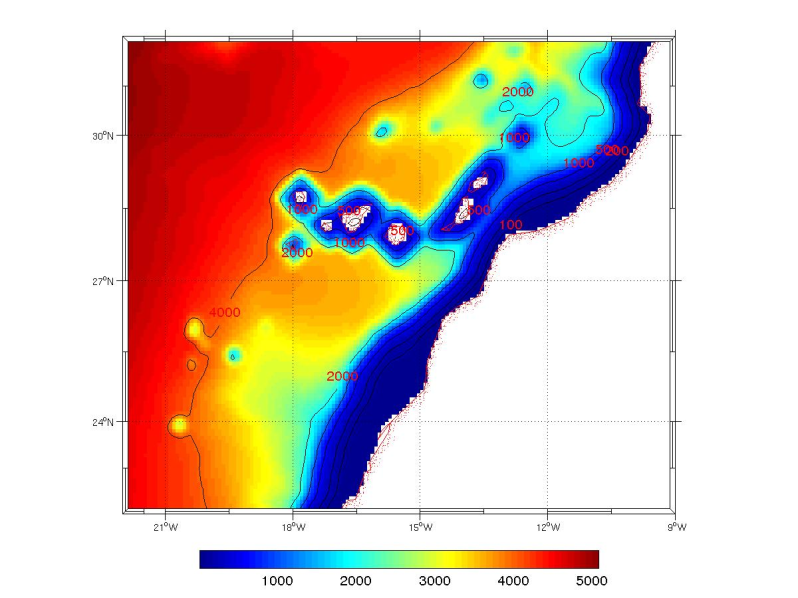 | Figure 2. GEBCO bathymetry of southern Morocco |
4. Validation of Results
The data used for validation are the sea surface temperature of NOAA (National Oceanic and Atmospheric Administration). These AVHRR observations (Advanced Very High Resolution Radiometer) are averaged over periods of 8 days at 01/01/2003 to 31/12/2006. For quantitative comparisons, an interpolation of satellite data on the grid of our field of study was made. To fill the missing points in the data file, it was necessary to proceed with an objective analysis (Package Roms_tools). Local comparisons focused on the following sites: Essaouira, Laayoune and Dakhla (Figure 3).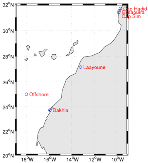 | Figure 3. The study region of West African. The circles indicate the locations of Aladin, in-situ and QuikSCAT comparisons |
4.1. Local Comparison
ROMS simulations forced by ALADIN and QuikSCAT winds are referred as respectively ROMS_ALADIN and ROMS_QSCAT.Temperatures simulated by the model in Essaouira and Laayoune are considered correct but their variability is significantly underestimated compared to that measured by the AVHRR instrument respectively with a standard RMSE of 1.44°C and 1.79°C with ROMS_ALADIN simulation and respectively 1.55°C and 1.80°C with ROMS_QSCAT simulation. The error relative to AVHRR data for both sites respectively 1.22°C and 1.47°C with the simulation ROMS_ ALADIN and 1.26°C and 1.44°C with ROMS_QSCAT simulation. The curve of ROMS_QSCAT simulation at Essaouira has a temporal disagree with the AVHRR measurement with a phase shift of a few remarkable days (Figure 4) whereas at Laayoune they have the same phase. Results are obtained with a correlation coefficient respectively of 59% and 60%. The discrepancies are due to the extrapolation of satellite data on land used in the model forcing. However, temperatures simulated by the model in Dakhla, have an average similar to the average of the measured temperatures. Indeed, modeling with QuikSCAT winds can reproduce the phase and amplitude of the cycle of the temperature measured by AVHRR with a high correlation coefficient of 78%. Simulation performed with the ALADIN winds present a temporal evolution disagree with the measurements. This can be explained by the inability of the ALADIN model to resolve the topographic complexity of the site Dakhla. In addition, the temperature curves simulated by ROMS in the three sites have the same trends as measured by AVHRR with a correlation coefficient generally important.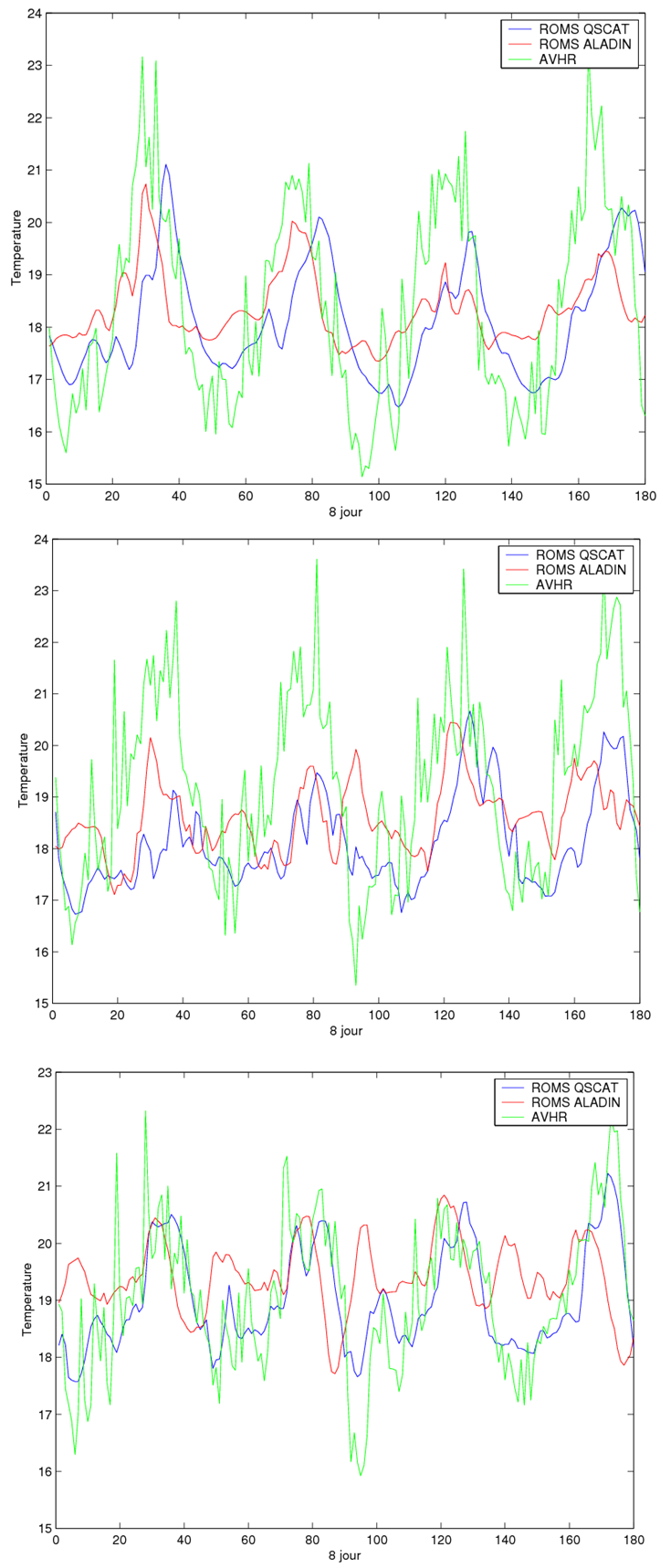 | Figure 4. Surface temperature in Essaouira (left), Dakhla (center) and Laayoune (right) for the period from 01/01/2003 to 31/06/2006 |
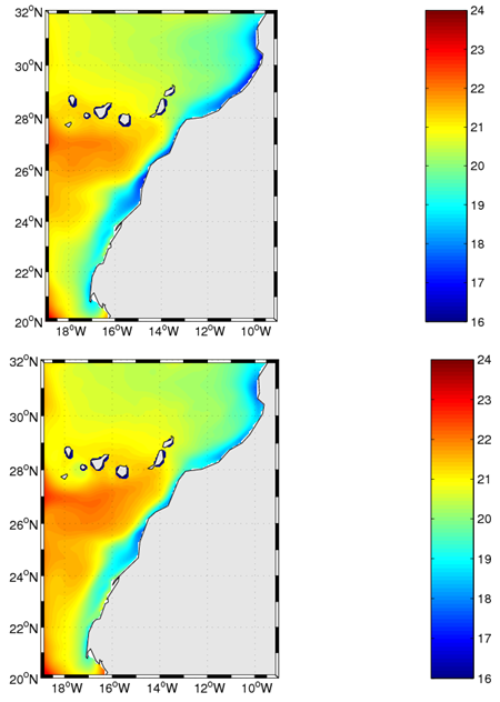 | Figure 5. Surface temperature with ROMS_QSCAT simulation (top) and ROMS_ALADIN simulation (bottom) for the period from 01/01/2003 to 31/12/2006 |
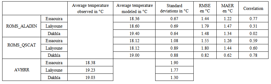 | Table 1. Statistical parameters of the surface temperature at Essaouira, Laayoune and Dakhla points |
4.2. Spatial Comparison
4.2.1. Annual Averages
With the annual spatial comparison, the distribution of surface temperatures ranging from high values the the deep ocean to low values near of coats highlighting the contribution of forcing on the coastal upwelling development. The configuration of the surface temperatures resulting from various simulations shows relatively few differences. However we noted colder coastal waters in the simulations ROMS_QSCAT and the warmer coastal waters are produced by ROMS_ALADIN simulations.
4.2.2. Seasonal Averages
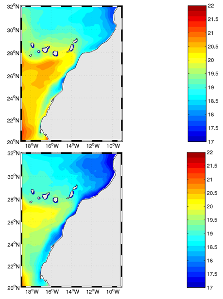
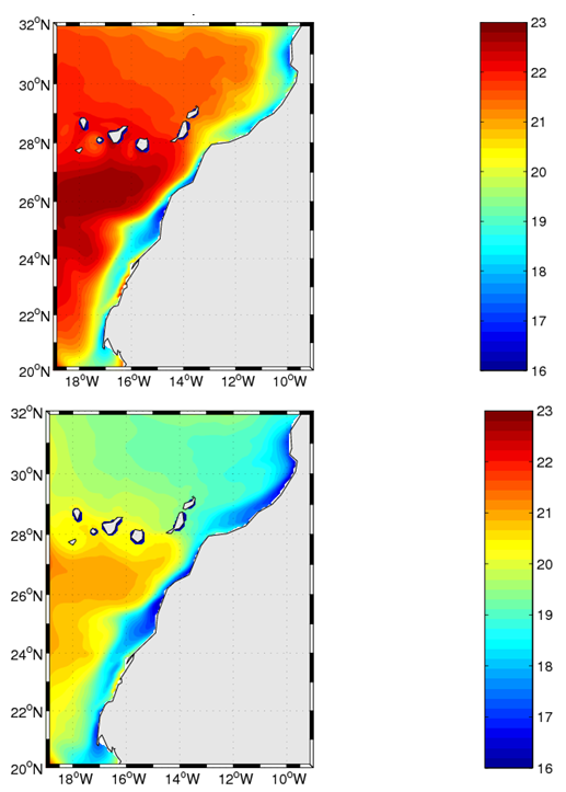
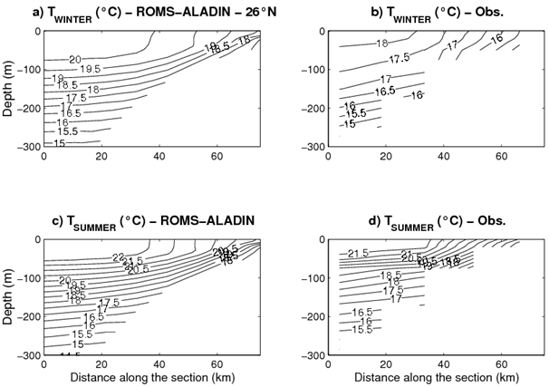
In similarity with the annual comparison, the seasonal distribution of surface temperatures ranged from high values in the deep ocean to low values at the coast highlighting the role of forcing on the development of coastal upwelling. Seasonality of the sea surface temperature is marked by warmer temperature in the deep ocean (in the subtropical gyre) than those obtained near coast. We also note colder coastal waters, in autumn, winter and summer, sharper in ALADIN simulation that in the QuikSCAT simulation, with an amplitude of the seasonal cycle between 17°C to 18°C at the coast. Furthermore, we note the presence of filament structures, visible in the autumn, with ROMS_ALADIN. This presence is much more marked during the autumn season when the simulations ROMS –ALADIN produces too much upwelling (Figure 6) and thus too energetic filaments and too long ones in their seaward extension. Indeed, recent studies of coastal upwelling systems have highlighted the existence of filaments near Cape Ghir (31° N), Cape Juby (28° N) and Cape Blanc (21° N) ([11], [3]). To better understand the variation of the sea surface temperature, we focus on the vertical temperature profile during the seasons of spring and summer on a meridional section at 26° N. The simulation period is from 2003 to 2006 and the period of observations from 1994 at 1997.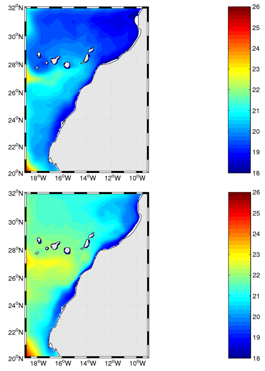 | Figure 6. Surface temperature with ROMS_ALADIN simulation (left) and ROMS_QSCAT simulation (right) in the fall (October, November and December) |
 | Figure 7. Surface temperature with ROMS_ALADIN simulation (left) and ROMS_QSCAT simulation (right) in winter (January, February and March) |
 | Figure 8. Surface temperature with ROMS_ALADIN simulation (left) and ROMS_QSCAT simulation (right) in the spring (April, May and June) |
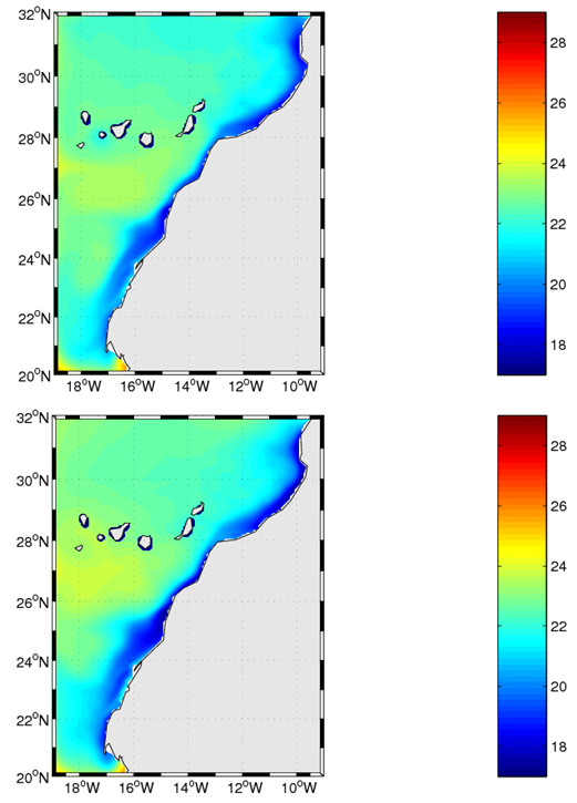 | Figure 9. Surface temperature with ROMS_ALADIN simulation (left) and ROMS_QSCAT simulation (right) summer (July, August and September) |
The simulated temperatures are overestimated compared to observed temperatures during the two seasons in both simulations, however they remain similar. The vertical temperature gradient during the spring is stronger in the simulations than in the observations. But, during the summer season, the temperature gradient is comparable between the two simulations and observations.
4.2.3. Analysis of Standard Deviations
The maximum standard deviation highlights areas of filamentation on the study area. The maximum is located slightly offshore because the filaments are generally anchored on caps; variability is low in caps but becomes stronger toward the open ocean more than the filament is unstable [9]. The simulation with the QuikSCAT winds produces a high variability, which is consistent with a stronger upwelling (produced by stronger winds) and more intense coastal currents producing stronger filaments. The temporal variability of the sea surface temperature is demonstrated by the standard deviations of the study period. The figures of the simulated temperature (Figure 12 and 13) illustrate the spatial variability of the sea surface temperature over the entire area, with a maximum standard deviation of 0.51°C for measurements and 0 47°C to 0.52°C for the various simulations over the entire study period ([10], [11]).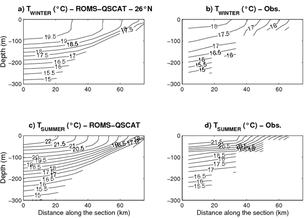 | Figure 10. Surface temperature with ROMS_QSCAT simulation (left) and observations (right) in the spring and summer |
 | Figure 11. Surface temperature of ROMS_ALADIN simulation (left), observations (right) in the spring and summer |
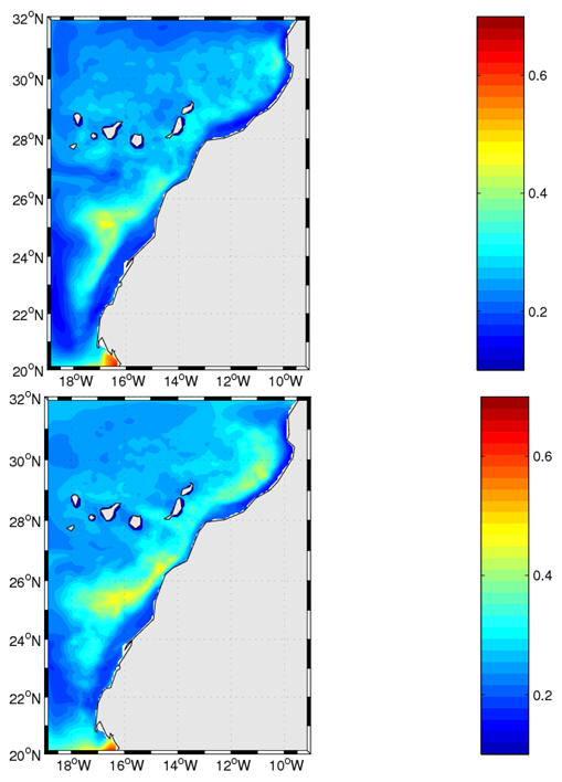 | Figure 12. Standard deviation of temperature with ROMS_ALADIN simulations (top) and ROMS_QSCAT (bottom) for the period from 01/01/2003 to 31/12/2006 |
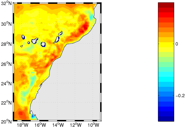 | Figure 13. Difference of standard deviation of temperature between simulations ROMS_QSCAT and ROMS_ALADIN for the period from 01/01/2003 to 31/12/2006 |
5. Conclusions
The majority of the upwelling events are reproduced on the coast. Using QUICKSCAT against ALADIN appears highlighted the variability of upwelling on the north coast. But it is on the south coast upwelling variability is highlighted by both simulations and dynamic forcing differences lead to differences in variability most remarkable. The wind in the product QuikSCAT extrapolated on the coast causes upwelling and too cold temperatures supported all along the coast, this is due to strong winds noticed with QuikSCAT winds. ALADIN simulates a classic effect at the Cape Peninsula Essaouira (cap SIM and cap Hadid) with light winds on the coast, which is why in ALADIN resolved structures upwelling mesoscale. Finally we conclude with two consequences: a remarkable upwelling along the coast on the one hand and a circulation towards the North related to the rotational wind Sverdrup relationship in the other hand. This circulation is found particularly in the south of the Canary Islands, where upwelling variability is important. Indeed, the wind as it passes by the islands creates atmospheric rotors in turn generating a cyclonic ocean circulation migrating north and strong variability accordingly.These simulations show that the upwelling is better quantified with the forcing of data meso-scale than forcing of climate data [12]. We note that although mainly with the figures of seasonal temperatures. Thus, we deduce the upwelling variability highlighted with data on temporal and spatial meso-scale than with the large-scale data.
ACKNOWLEDGEMENTS
This research has been supported by the National Direction of meteorology (DMN) of Morocco, and by LPO (Laboratoire de Physique des Océans, Brest, France). We would to thank Nicolas Grima for his recommendations and help. We also thank D. Dagorne for the interesting discussions and suggestions.
References
| [1] | ALADIN International Team, “The ALADIN project: Mesoscale modelling seen as a basic tool for weather forecasting and atmospheric research”, WMO Bulletin 46/4 , pp. 317–324, 1997. |
| [2] | B. Barnier, L. Siefridt and P. Marchesiello, “Thermal forcing for a global ocean circulation model using a three-year climatology of ECMWF analyses”, J. Mar. Syst., 6, 363-380, 1995. |
| [3] | E. Barton, “Eastern boundary of the North Atlantic: Northwest Africa and Iberia. Coastal segment (18, E)”, In: Robinson, A., Brink, K.H. (Eds.), The Sea, vol. 11. John Wiley & Sons Inc., pp. 633–657, 1998. |
| [4] | Y. Chao, Z. Li, J.C. Kindle, J.D. Paduan, F.P. Chavez, “A High- Resolution Surface Vector Wind Product for Coastal Oceans: Blending Satellite Scatterometer Measurements with Regional Mesoscale Atmospheric Model Simulations”, Geophysical Research Letters, 30(1), 1013. doi:10.1029/ 2002GL015729, 2003. |
| [5] | P. Cury, C. Roy, “Migration saisonnière du thiof (Epinephelus aeneus) au Sénégal : influence des upwellings sénégalais et mauritanien“, Oceanol. Acta, 11, 1, 32-33, 1987. |
| [6] | C. Roy, R Mendelssohn, “The development and the use of a climatic database for CEOS using the COADS dataset.” 1998. |
| [7] | A. Bentamy, K.B. Katsaros, A.M. Mestas-Nuñez, W.M. Drennan, E.B. Forde, H. Roquet, “Satellite estimates of wind speed and latent heat flux over the global oceans.” J. Climate, 16, 637-656, 2003. |
| [8] | [Online].Available:IRD[http://www.mpl.ird.fr/suds-en-ligne/ecosys/upwelling/canaries.htm]. |
| [9] | P. Marchesiello, J.C. McWilliams, A. Shchepetkin, “Equilibrium structure and dynamics of the California Current System.” J. Phys. Oceanography., 33, 753-783, 2003. |
| [10] | A. Moujane, A. Bentamy, M. Chagdali, S. Mordane, “Analysis of high spatial and temporal surface winds from Aladin model and from remotely sensed data over the Canarian upwelling region.” Accepté le 11 mars 2011, mis en ligne le 30 mai 2011 © Revue Télédétection, 2011, vol. 10, n° 1, p. 11-22, 2011A. |
| [11] | A. Moujane, M. Chagdali, B. Blanke, S. Mordane, “Impact des vents sur l’upwelling au sud du Maroc ; apport du modèle ROMS forcé par les données ALADIN et QuikSCAT”, Bulletin de l’Institut Scientifique, Rabat, section Sciences de la Terre, 2011, n°33, p. 53-64, 2011B. |
| [12] | A. Moujane, M. Chagdali, S. Mordane, “L’apport des vents climatologiques de COADS et QUIKSCAT dans la modélisation de la SST au Sud du Maroc.” Accepté le 17 décembre 2013, publié le mois de mars 2014 GEO OBSERVATEUR | N° 21, Mars/Marsh 2014, p. 83-91, 2014. |
| [13] | A.F. Shchepetkin, J.C. McWilliams, “Regional Ocean Model System: a split-explicit ocean model with a free-surface and topography-following vertical coordinate.” Ocean Modelling 9, 347-404, 2005. |
 Abstract
 Reference
 Full-Text PDF
 Full-text HTML