Ana C. Pedraza De Marchi 1, 2, Marta E. Ghidella 3, Claudia N. Tocho 1
1Universidad Nacional de La Plata, Facultad de Ciencias Astronómicas y Geofísicas, La Plata, 1900, Argentina
2CONICET, Concejo Nacional de Investigaciones Científicas y Técnicas, Argentina
3Instituto Antártico Argentino, Buenos Aires, C1064AAF, Argentina
Correspondence to: Ana C. Pedraza De Marchi , Universidad Nacional de La Plata, Facultad de Ciencias Astronómicas y Geofísicas, La Plata, 1900, Argentina.
| Email: |  |
Copyright © 2014 Scientific & Academic Publishing. All Rights Reserved.
Abstract
We have tested and used two methods to determine the Bouguer gravity anomaly in the area of the Argentine continental margin. The first method employs the relationship between the topography and gravity anomaly in the Fourier transform domain using Parker’s expression for different orders of expansion. The second method computes the complete Bouguer correction (Bullard A, B and C) with the Fortran code FA2BOUG2. The Bouguer slab correction (Bullard A), the curvature correction (Bullard B) and the terrain correction (Bullard C) are computed in several zones according to the distances between the topography and the calculation point. In each zone, different approximations of the gravitational attraction of rectangular or conic prisms are used according to the surrounding topography. Our calculations show that the anomaly generated by the fourth order in Parker’s expansion is actually compatible with the traditional Bouguer anomaly calculated with FA2BOUG, and that higher orders do not introduce significant changes. The comparison reveals that the difference between both methods in the Argentine continental margin has a quasi bimodal statistical distribution. The main disadvantage in using routines based on Parker's expansion is that an average value of the topography is needed for the calculation and, as the margin has an abrupt change of the topography in the continental slope area, it causes a bimodal distribution. It is worth noticing that, as expected, the most important differences between both methods are located over the continental slope both in complex structures such as part of the shared margin, as well as in isolated points where there are contributions from short wavelength or rugged topography.
Keywords:
Bouguer anomaly, Argentine continental margin, Parker’s expansion, Grdfft3, Gravfft1, FA2BOUG
Cite this paper: Ana C. Pedraza De Marchi , Marta E. Ghidella , Claudia N. Tocho , Analysis of Different Methodologies to Calculate Bouguer Gravity Anomalies in the Argentine Continental Margin, Geosciences, Vol. 4 No. 2, 2014, pp. 33-41. doi: 10.5923/j.geo.20140402.02.
1. Introduction
The Argentine passive margin is of rifted volcanic type. This classification is based primarily on the presence of volcanic wedges buried beneath the continental slope, manifested by seismic data as seaward dipping reflector sequences (SDRs) [1], [12].Distinct along-margin variations in architecture, volume, and width of the SDRs wedges are probably related to margin segmentation [1]. Authors have suggested that the margin can be divided, at least, in four compartments bounded by the Falkland transfer (Falkland-Malvinas Fracture Zone), Colorado transfer, Ventana transfer and the Salado transfer. They use the term transfer zone to describe crustal lineaments or discontinuities in the margin architecture and they have interpreted it as old zones of weakness controlling the onset of Upper Cretaceous seafloor spreading, which may be linked to recent fracture zone. The presence of such transfer zones and their influence on the Bouguer gravity anomaly of the region deserves a comprehensive study which is beyond the scope of this paper. The Bouguer anomaly takes into account the effect of the gravitational attraction of the mass between the vertical datum, i.e., the ellipsoid or the geoid, and the gravity station. Bouguer anomaly is used in geophysical modelling and interpretation of continental basins and lake environments.However, most papers about margins and oceans use the free-air anomaly for gravity analysis instead. The reason for this is that the Bouguer anomaly is not as necessary as it is in continental areas, where topographic effects normally mask the contribution of the crustal features below. Nevertheless, there are still interpreters and methods that need the Bouguer anomaly also in maritime regions. We have found that in those marine studies that use the Bouguer anomaly, nothing is said about the method employed in the calculation, possibly because the authors consider it as straightforward and very simple.This paper intends to fill that void, as we consider it is not that simple. We have found that calculating the Bouguer anomaly in marine areas is not as straightforward as tacitly assumed, and consequently we experimented on the methods to use. Therefore, in this paper we describe our numerical experimentation, which consists in the comparison of two different methodologies to compute Bouguer gravity anomalies in the margin. The first one is based on the Parker's expansion to take into account the topographic effects, and the second one is a calculation of the complete Bouguer gravity anomaly following a traditional rigorous methodology generally designed for continental regions but which has been extended to marine zones.In marine areas, the Bouguer correction involves replacing the density of water with a rocky material, usually with density of 2670 kg/m3. In deep ocean waters, this replacement produces large positive gravity anomalies with a steep gradient for interpretation. This is the reason why using free-air anomalies offshore is actually more appropriate [6].In geophysics the Bouguer reduction is used in continental areas in an attempt to remove the gravitational effects of the topographic masses and the high correlation between free-air gravity anomalies and elevation. The incorrect estimation of the density of the topographic masses causes distortions in the Bouguer gravity anomalies. In geodesy, Bouguer reduction is used to smooth the gravity field to avoid aliasing during the interpolation and gridding of gravity data. [4], [5]. We have used three routines to obtain the Bouguer anomaly: grdfft from the Generic Mapping Tools (GMT) [14], gravfft written by Joaquim Luis [15], which performs mathematical operations on grid files in the wavenumber or frequency domain based on Parker's expansion, and the third is FA2BOUG, a Fortran 90 program developed by Fullea et al. [3], it obtains the complete Bouguer anomaly. However, although FA2BOUG has refined approaches in the calculation of the classic Bouguer anomaly, with gravfft up to some specified order we obtain a suitable calculation for a regional scale computation and the comparison reveals that the difference between FA2BOUG and gravfft up to four order follows a bimodal distribution, which maximum frequency is 1.8 mGal and the bias is 1.1 mGal. We can consider that the difference is found between ±1.8 mGal, which is acceptable taking into account that they are very different methodologies of calculation. With this result, we are able to assume that we can confidently use other routines that are based on the Fourier transform and work on the wavenumber domain for other gravity interpretation methods such as our general objective of understanding the isostasy of the margin and adjacent ocean, as well as other studies.
2. Methodology
2.1. Method 1. Using Parker’s Expression
The gravity effect of uncompensated sea-floor topography (bathymetry) at sea level can be written to first order as (Watts, 2001):  | (1) |
where ρc y ρw are the densities of the sea-floor topography and sea water, respectively, G is the Newton gravitational constant, H(k) is the Fourier transform of an undulating sea-floor topography and d is the mean water depth. Equation (1) assumes that in the wave number domain, the gravity anomaly is linearly related to the bathymetry.The complete expression for the gravity effect of uncompensated sea-floor topography at sea level is given by Parker, as in [10], as: | (2) |
where n is the order. When n=1 in equation (2), we get the expression given in (1) which corresponds to a first-order approach that is only an approximation of equation (2). High-order terms in the series expansion of the gravity anomaly are present in (2). Computation of the Bouguer Anomaly Using Method 1The Bouguer anomaly is computed following these three steps: 1) Use the programs grdfft and gravfft of GMT, the gravity effect of the interface water-crust (wc) can be computed with the expression given in (1) and (2), respectively; gravfft allows computing equation (2) up to higher order.2) Remove the gravity effect of the interface water-crust computed in the step 1) from the observed free-air gravity anomaly. 3) Compute the Bouguer correction as the gravity effect of a slab of density contrast between water and crust of infinite radius and thickness equal to the mean height of the bathymetry and added to step 2).  | (3) |
where ΔgFA is the free-air gravity anomaly, wc is the gravity effect of the interface water-crust computed in step 1) and wcslab is the gravity effect of the slab calculated in 3).
2.2. Method 2. Complete Bouguer Anomaly
The Bouguer anomaly is obtained using data grids of bathymetry, topography and free air anomalies. The complete Bouguer correction is calculated in three steps: correction of the Bouguer slab (Bullard A), which approximates the topography or local bathymetry with a plate of infinite lateral extension of constant density and thickness equal to the elevation of the point with respect to the sea level; curvature correction (Bullard B), which replaces the Bouguer plate by a spherical layer of the same thickness and surface 166,735 km [7] and the topographic correction (Bullard C), which consists of the effects of the surrounding topography above and below the station.Computation of the Bouguer Anomaly Using Method 2The Fortran program developed by Fullea FA2BOUG [3] calculates Bouguer anomaly for land and sea points. The input is adapted for the use of sets of global grids of free air gravity anomalies and elevation/bathymetry. The program calculates the corrections Bullard A, Bullard B and Bullard C in several zones (near, intermediate and distant) depending on the horizontal distance (R) between topography and the point where the complete Bouguer anomaly is calculated. The topography is digitized through a set of squares flat-topped prisms centered at each point of a Digital Elevation Model (DEM) and height elevation given by the DEM. FA2BOUG calculates the full topographic effect (Bouguer plate plus curvature-correction plus topographic correction). For marine areas FA2BOUG defines three areas of computation:1) an inner zone (R < Δxi/2). The inner zone consists of a  side square centred on the calculation point. The inner contribution to the full Bullard correction is calculated in two steps. In the first one, the vertical attraction is computed due to an inner flat-topped prism with lateral extension equal to the size of the inner zone and height equal to the elevation of the calculation point. In the second one, the inner zone is divided into four quadrants with a constant slope upwards or downwards from its vertex to the calculation point, i.e. a quarter of a conic prism with its vertical axis through the calculation point and height equal to the difference between the elevation of the surrounding topography and height to the elevation of the calculation point [3].2) an intermediate zone (Ri > R > Δxi/2), Δxi is the grid step. The vertical attraction produced by a rectangular prism is calculated with the analytical formula in Cartesian coordinates given by Nagy et al. [9].3) and a distant zone, (Rd > R > Ri). In this zone the spherical harmonic expansion of the gravitational potential of a right rectangular prism is considered [8] to avoid numerical instabilities.In 1), 2) and 3) Ri is the limit of the intermediate zone (20 km), chosen by a series test that evaluates the compromise between accuracy and the calculation time [3], Rd is the limit of the distant area (167 km) and Δxi the intermediate zone grid step (2 km approximately, it is obtained from the resolution of the grid step in arc minutes (1')).
3. Results
3.1. Study Area and Maps of the Differences
The study area corresponds to a section of the Argentine continental margin between latitudes 39.5°S and 48.25°S and longitudes 63°W and 51°W. (Figure 1). For the calculation we use a one degree extended area in all map boundaries to avoid the typical edge effects that may arise when working with Fourier transform.Free-air gravity anomalies and elevation data, i.e. topography and bathymetry, come from the global satellite altimetry data compilation V18.1 and V14.1, respectively by Sandwell and Smith [12]. The resolution of both versions is 1’x1’.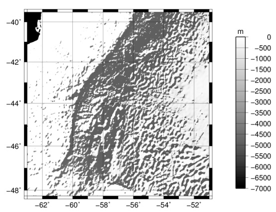 | Figure 1. Shaded image of the bathymetry data in the area under study (illumination is from the NW) (Sandwell y Smith, 2009) |
Figure 2 shows the Bouguer gravity map using a) FA2BOUG and b) gravfft to order 4. The general trend of inverse correlation between these Bouguer gravity anomaly maps and bathymetry (Figure 1) can be observed. Positive Bouguer anomaly values are found in the Atlantic Ocean and we can observe the very abrupt gradient around the shelf break area, which changes along the margin following its main structure.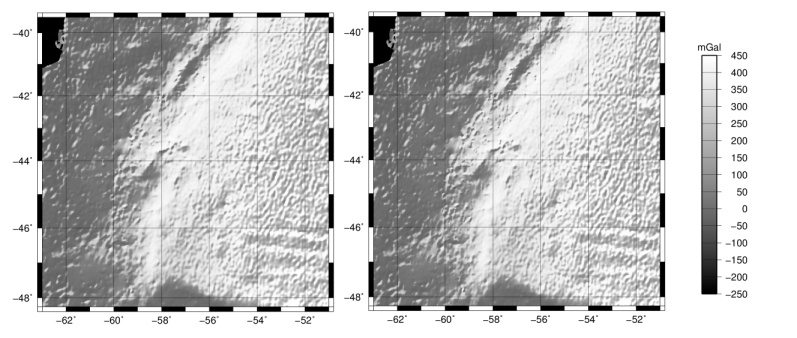 | Figure 2. Bouguer gravity map using the programs a) FA2BOUG, b) gravfft to order n = 4 |
Figure 3 shows the comparison of Bouguer anomalies computed using the programs grdfft and gravfft up to degree n=4, respectively with respect to FA2BOUG. In the Figure 3a we can observe the bimodal behavior of the difference, which is characterized by a positive value in the deep ocean area and a negative value in the shallow ocean area.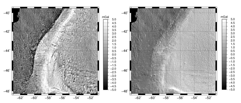 | Figure 3. Bouguer gravity map using the programs a) FA2BOUG, b) gravfft to order n = 4 |
The maps of Figure 4 displays the differences between different orders in Parker’s expansion. On (a) we see that the difference between n=4 and n=1 (grdfft uses n=1), is a lot correlated with the seafloor topography, whereas in (b) (n=5 minus n=4) we observe that for higher orders the differences still exists, still are correlated with the morphology, but the effect is minor or negligible.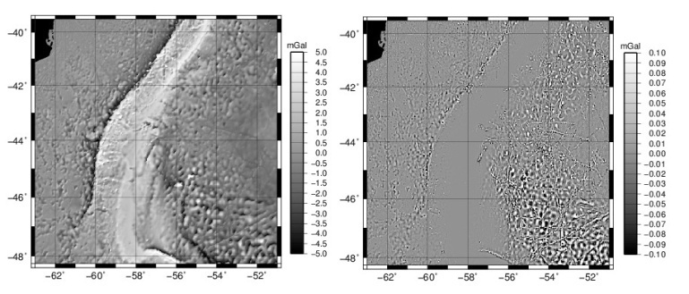 | Figure 4. Differences between a) gravfft n=4 and grdfft, b) gravfft n = 5 and gravfft n = 4 |
3.2. Statistic Information from the Differences
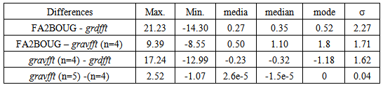
The statistics of Table 1 only correspond to the oceanic area; we have used grdlandmask of GMT, which keep the nodes of the grid only over water.Analyzing statistical information in Table 1, we can conclude that the increment of the orders from order n=4 in the Parker’s expansion does not introduce significant changes compared to the anomalies computed with FA2BOUG. However, spatial differences can be noticed in the calculation of the Bouguer anomaly between orders 5 and 4 with gravfft, as observed in the graph in Figure 4b and in Table 1. Calculation of Bouguer anomalies with the development of Parker up to 4 is enough to make the comparison with the calculated ones with the anomalies calculated by FA2BOUG.Table 1. Statistics of the differences of Bouguer anomalies computed with gravfft, grdfft, FA2BOUG and their comparison. Unit: [mGal]
 |
| |
|
As the arithmetic mean parameter of a set of data is very sensitive to extreme values, the median of the differences is calculated considering that it is more appropriate to describe distributions of data that do not have a normal trend. The median shows the symmetry of the distribution around the amount of data and the mode describes the difference for which the rate is maximum. The differences of the anomalies computed with Parker's order four or higher and FA2BOUG follows almost a bimodal distribution (Figure 5a and Figure 6a) and shows a marked bias; besides it is different between various degrees of Parker that are centered, which much lower a bias (Figure 5b and Figure 6b).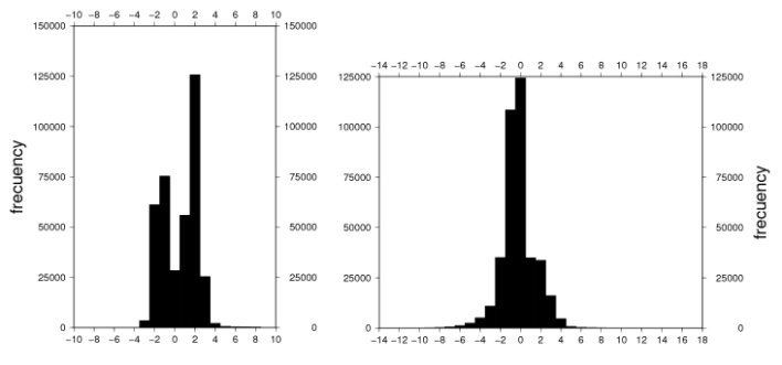 | Figure 5. Histograms of a) FA2BOUG minus gravfft up to order n=4, b) gravfft up to order n=4 minus grdfft |
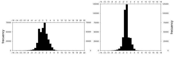 | Figure 6. Histograms of a) FA2BOUG minus grdfft, b) gravfft up to order n=5 minus grdfft |
Since both methods employed in this study are so different, it is acceptable that differences are commonly between ±1.8 mGal, which is observed in Table 1 and in Figure 5a. This Figure shows two main frequencies, which are around values 1.8 mGal and -1.5 mGal. The first one is associated with the points in the abyssal plain area (deep ocean area); the second one is associated with the points in the continental terrace (shallow ocean area) before crossing the continental slope. On Figure 5a we can observe that the difference has three main behaviours; it is positive in the deep ocean area where the main frequency is around 1.8 mGal (Figure 7a), negative in the shallow ocean area where the main frequency is around -1.5 mGal (Figure 7c), and the rest is mainly distributed in the continental slope area of the passive and sheared margins (Figure 7b).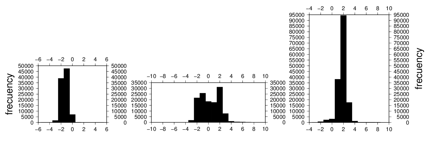 | Figure 7. Histograms FA2BOUG minus gravfft up to order n=4 in three longitudinal areas, a) -63º≤λ≤-60º b) -60º≤λ≤-56º c) -56º≤λ≤-51º (λ is geographical longitude) |
This behaviour represents the main disadvantage of the routines grdfft and gravfft, which are based on Parker's expansion, because they need an average value of the topography to be applied and the margin has an abrupt change of the topography in the continental slope area, which is cause the bimodal distribution. We could try dividing the area in zones and then overlapping them in one grid, but the problems are how to deal with the limit of the continental slope and how to determine which is the best way to overlap such zones, and these represent a numeric time consuming complication.
3.3. Two Special Profiles of Bouguer Anomalies
Two profiles at latitudes 45.32°S and 48°S, respectively are displayed in Figure 8. The profiles are represented as a function of the distance to the first point of the profile. The upper curve represents the Bouguer anomaly calculated with the three programs: FA2BOUG, grdfft and gravfft up to order n = 4 and the lower curve represents the corresponding bathymetry. Discrepancies between the calculation methodologies are almost negligible except for specific cases like the ones shown in Figure 8.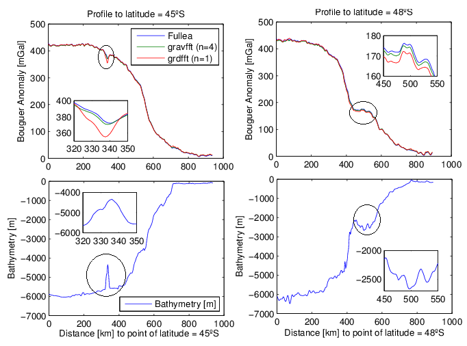 | Figure 8. Longitudinal profiles at latitude a) 45.32°S, b) 48° S (b) |
The area of the largest discrepancy is generated by the contribution of the high wavelength of the sea-floor topography as in the profiles on Figure 8a, to latitude 45.32ºS, where there is a seamount 2000 meters height [2], which causes the deviation between curves computed with grdfft respect to the others and the differences are approximately of 20 mGal (accordance to Table 1 and Figure 8a). Other discrepancies might be due to blunders in the Sandwell model bathymetry data but, in general, they are due to the sudden change of the gradient of the sea-floor topography, i.e. very abrupt slope changes generate pronounced Bouguer anomalies complicated for interpretation. That is why free air gravity anomalies are so often used for interpretation of marine areas [5].In the case of Figure 8b, the profile crosses an important submarine canyon system conditioned by an active dynamic of the water mass of Antarctic origin, which has been favored by great sedimentary thickness conforming one contourite depositional system [2]. We can appreciate that the contribution of the short wavelength of the sea-floor topography is lower than the case of Figure 8a, but it is enough to provide a local differentiation of the three curves.
3.4. Differences Cross Plot
Three cross plots are showed on Figure 9, where the differences between calculations methods versus bathymetry are shown. On average, it can be said that the difference of the Bouguer gravity anomaly up to degree n=4 and FA2BOUG are linearly correlated with the sea-floor topography (Figure 9c). Even though in Figure 9 there are values which do not have a polynomial behavior (Figure 9a and 9b) or linear behavior (Figure 9c), the spatial distribution of the high discrepancies between the Bouguer anomaly calculated with two different methodologies are filtered and shown in Figure 10 and Figure 11. | Figure 9. Cross plots of: a) FA2BOUG minus grdfft, b) gravfft up to degree n=4 minus grdfft, c) FA2BOUG minus gravfft up to degree n=4 vs. bathymetry |
3.5. Spatial Distribution of Outliers
Continuing with the analysis of the differences in the grids of Figures 3 and 4, it can be shown more appropriately that for high orders of the Parker’s expansion the independence with the morphology of the margin is greater. We are interested in learning where the outlier values are spatially distributed. The differences over 5 mGal (values that are out of the main distribution of the frequency, Figures 5a and 9c) are located mostly on the edge of the slope (Figure 10b and Figure 11). It is noted that in the comparison between the classic method that use Fullea in FA2BOUG and gravfft based on the development of Parker's up to order n = 4 are both sensitive to structures like the Falkland transfer zone where the residual difference between both in such zone (Figure 10a) has decreased respect to the residual difference between FA2BOUG and grdfft based on the development of Parker's up to order n = 1, it is depicted in Figure 11; which shows that gravfft (n=4) and FA2BOUG are able of detecting this structure (Figure 10a).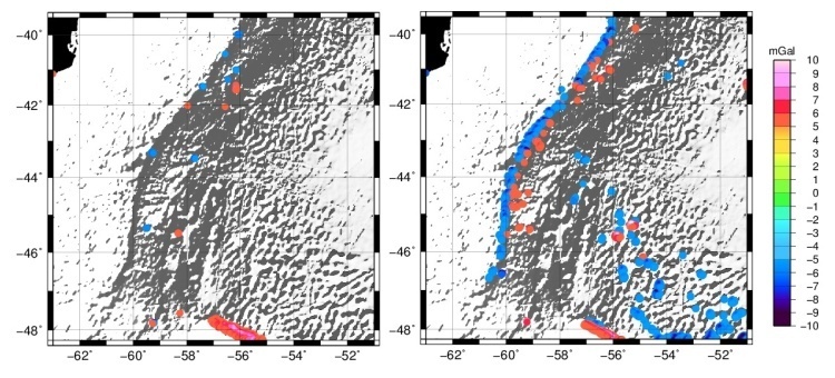 | Figure 10. Differences between a) FA2BOUG and gravfft n=4 > 5 mGal, b) gravfft n=4 and grdfft > 5 mGal |
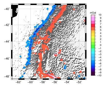 | Figure 11. Differences between FA2BOUG and grdfft > 5 mGal |
4. Conclusions
We have presented a comparison of two different methodologies to compute Bouguer gravity anomalies in the Argentine continental margin. One method uses Parker’s expansion incorporated into the programs grdfft or gravfft and the other method was developed by Fullea in its FA2BOUG program. We need to clarify that in neither case, sediment thickness grids of the region and their contribution to Bouguer anomaly with the corresponding density contrast were considered, because the paper is focused on the study the differences between both methods. A more refined model to calculate the Bouguer anomaly would take into account the sediment thickness, sometimes that can be easily implemented in method 1.The methodology of calculation proposed by FA2BOUG is rigorous and robust; however, similar results can be achieved faster using Fourier transform routines such as gravfft. We conclude that both methods are equivalent in the task of approximating the Bouguer anomaly, and Parker’s expansion up to order 4 and FA2BOUG are also sensitive to complex structures such as the Falkland/Malvinas transfer zone.Increasing the order in Parker’s expansion, a better approximation of the Bouguer anomaly is obtained, which up to order 4, constitutes an improvement compared with the calculation using FA2BOUG. However, the statistical comparison reveals than the difference has a bimodal behavior, as it is positive in the deep ocean area where the main frequency is around 1.8 mGal and negative in the shallow ocean area where the main frequency is around -1.5 mGal. The main disadvantage on using routines based on Parker's expansion in the margin area is that an average value of the topography needs and to be used and the margin has an abrupt change of the topography in the continental slope area, which is the cause of the bimodal distribution of the difference.We observed profiles where the discrepancies between methods lie in the regions where the continental slope presents local variations of very high frequency or regions where the continental slope is very steep. Also abrupt changes in slope may not be well represented, but nevertheless good enough for a number of studies.The difference between the Bouguer anomaly calculation methodologies is on average highly correlated with the abrupt changes in topography, as we could expect. But the Fourier methods (using grdfft and gravfft), are simpler for the incorporation of sediment loading and the treatment of large oceanic areas.
ACKNOWLEDGEMENTS
The free-air gravity anomaly are Public domain and we take it from the website [18] (Sandwell, 1997; Sandwell, 2009).The maps and graphs have been drawn using the Generic Mapping Tools (GMT) open source software (Wessel and Smith, 1998).
References
| [1] | Franke D, S. Neben, S. Ladage, B. Schreckenberger, and K. Hinz, 2007. Margin segmentation and volcano-tectonic architecture along the volcanic margin of Argentina/Uruguay, South Atlantic, Elsevier, Marine Geology, 244, 46-47. |
| [2] | Fernandez-Molina F. J., M. Paterlini, R. Violante, P. Marshall, L. Somoza and M. Rebesco, 2009. Contourite depositional system on the Argentine Slope: An exceptional record of the influence of Antartic wáter mases, Geology, vo. 37, no. 6, 507-510. |
| [3] | Fullea J., M. Fernandez and H. Zeyen, 2008. FA2BOUG-A FORTRAN 90 code to compute Bouguer gravity anomalies from gridded free-air anomalies: Application to the Atlantic-Mediterranean transition zone, Computers & Geosciences, vol. 34, p. 1665-1681. |
| [4] | Hackney, R.I., and W.E. Featherstone, 2003. Geodetic versus geophysical perspectives of the gravity anomaly. Geophys. J. Int., July 2003, v.154, p. 35-43. |
| [5] | Heiskanen,W.A.and Moritz, H., 1967. Physical Geodesy, Freeman, San Francisco. |
| [6] | Keller, G. R., T. G. Hildenbrand, W. J. Hinze, X. Li, D. Ravat, M. Webring, 2006. The quest for the perfect gravity anomaly: Part 2 — Mass effects and anomaly inversion, SEG Expanded Abstracts 25, p. 864-868. |
| [7] | LaFehr, T. R., 1991. An exact solution for the gravity curvature, Bullard B, Geophysics, vol. 56, no. 8, p. 1179-1184. |
| [8] | McMillan, W.G., 1958. The theory of Potential. Dover Publisher, New York, 469 pp. |
| [9] | Nagy, D., G., Papp, J. Benedek, 2000. The gravitational potential and its derivatives for the prism. Journal of Geodesy, vol. 74, p.552-560. |
| [10] | Parker, R. L., 1973. The rapid calculation of potential anomalies, Geophys. J. R. Ast. Soc., vol. 31, p. 447-455. |
| [11] | Sandwell, D., 1997. Marine gravity anomaly from Geosat and ERS 1 satellite altimetry, Journal of Geophysical research, vol. 102, no. B5, p. 10,039-10,054. |
| [12] | Sandwell, D., 2009. Global marine gravity from retracked Geosat and ERS-1 altimetry: Ridge segmentation versus spreading rate, Journal of Geophysical Research, vol. 114, B01411, doi:10.1029/2008JB006008, 2009. |
| [13] | Schnabel, M., D. Franke, M., Engels, K. Hinz, S. Neben, V. Damm, S. Grassmann, H. Pelliza, P. R. Do Santos, 2008. Tectonophysics, v.454, p. 14-22. |
| [14] | Watts, A. B., 2001. Isostasy and flexure of the lithosphere, Cambridge University Press. |
| [15] | Wessel, P. and W. H. F. Smith, 1991. Free software helps map and display data, EOS Trans. AGU, 72, 441. |
| [16] | http://w3.ualg.pt/~jluis/software.htm, 2011. |
| [17] | http://www.sciencedirect.com/science/article/pii/S0098300408001027, 2010. |
| [18] | http://topex.ucsd.edu/cgi-bin/get_data.cgi,2011. |
 Abstract
 Reference
 Full-Text PDF
 Full-text HTML