1. Introduction

Modeling of dynamic processes leading to an earthquake is one of the main concerns of seismologist. Two consecutive seismic events in a seismically active region are usually separated by a long aseismic period during which slow and continuous aseismic surface movements are observed with the help of sophisticated measuring instruments. Such aseismic surface movements indicate that slow aseismic change of stress and strain are occurring in the region which may eventually lead to sudden or creeping movements across the seismic faults situated in the region.

It is therefore seems to be an essential feature to identify the nature of the stress and strain accumulation in the vicinity of seismic faults situated in the region by studying the observed ground deformations during the aseismic period. A proper understanding of the mechanism of such aseismic quasi static deformation may give us some precursory information regarding the impending earthquakes.

A pioneering work involving static ground deformation in elastic media were initiated by ([8], [9]), ([21]), ([2]), ([3]),([6]), ([23]). Reference ([22]) has discussed various aspects of fault movement in his book. Reference ([5]) has discussed stress accumulation near buried fault in lithosphere-asthenosphere system.

In most of these studies the medium were taken to be elastic and /or viscoelastic, layered or otherwise. We now focus on some of the reasons of consideration of viscoelastic layer over viscoelastic half space model.

The laboratory experiments on rocks at high temperature and pressure indicates the imperfect elastic behavior of the rocks situated in the lower lithosphere and asthenosphere.

Investigations on the post-glacial uplift of Fennoscandia and parts of Canada indicate that at the termination of the last ice age, which happened about 10 millennia ago a 3km. ice cover melted gradually leading to upliftment of the regions .Evidence of this upliftment has been discussed in Fairbridge (1961), Schofield (1964), Chathles (1975), if the Earth were perfectly elastic, this deformation would be managed after the removal of the load, but it did not happened, indicating that the Earth crust and upper mantle is not perfect elastic but rather viscoelastic in nature.

Therefore in the present case we consider a long strike-slip fault situated in a viscoelastic layer over a viscoelastic half -space which is surface breaking in nature. The medium is under the influence of tectonic forces due to mantle convection or some related phenomena. The fault undergoes a creeping movement when the stresses in the region exceed certain threshold values.

2. Formulation

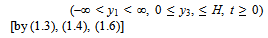
We consider a long strike-slip fault F width D situated in a viscoelastic layer over a viscoelastic half space of linear Maxwell type.

We choose our rectangular Cartesian coordinates (y₁, y₂, y₃) such that, the free surface is the plane y₃ = 0 the fault F₁ is in the plane y₂ = 0, y₁-axis is perpendicular to plane of the fault and y₃ axis pointing downwards as shown in the Fig: 1.Since our model is a viscoelastic layer of finite depth say H, over a viscoelastic half space.

∴ The interface is the plane y₃ = H.

We consider the fault F₁ in the region y₂ = 0, 0 < y₃ < D₁ < H

The half space is y₃ > H.

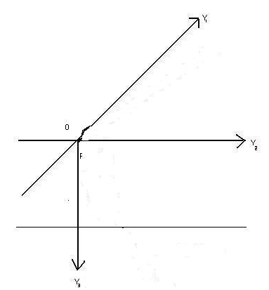Figure 1. Section of the model by the plane y1=0

Since we are concentrating 2D problem in which the length of the fault is large compared to the depth of it.

We take displacement, stress, strain to be in dependent of y₁ and dependent on y₂, y₃, t where‘t’ is the time measured after the establishment of aseismic state.

Let the components of displacement, stress and strain in the layer M₁ be u₁, τ¹₁₂, τ¹₁₃, e ¹₁₂, e ¹₁₃ respectively and in the half space M₂ be u₂, τ ²₁₂, τ ²₁₃,

e ²₁₂, e ²₁₃.

Since we are considering strike-slip movement only. we are not considering the other components of displacements, stresses, strains (u₂, u₃, τ₂₂, τ₂₃, etc.)

In our model M₁ is isotropic-homogeneous layer of rigidly modus μ₁, effective viscosity η₁ (say).M₂ is another isotropic homogeneous half space of rigidity modulus μ₂ and effective viscosity η₂ (say).

2.1. Constitutive Equations

For perfect elastic body we know as soon as the stress is removed. The strain also disappears but for viscoelastic body, the strain does not at once remove.

To incorporate the viscoelastic effects stress-strain relations of a slightly different form have been suggested.

We have the constitutive equations (i.e., stress -strain relation) as, for the layer M_1,

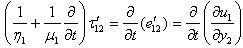(1.1)

(1.2)

(−∞ < y₂ < ∞, 0 < y₃ < H, t > 0)

For the half space M₂

(1.3)

(1.4)

(−∞ < y₂ < ∞, y₃ > H, t> 0)

2.2. Stress Equation of Motion

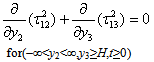
We have the stress equation of motion as

Since displacement, stress and strain are independent of y₁ therefore the stress equation becomes,

,

ρ= average density of M₁

Since our observation is in the aseismic period while the order of displacement is 10−⁴ c.g.s. unit or less.

∴ The inertial term is extremely small. Therefore, we neglect it.

Stress equation of motion for the layer M₁ is

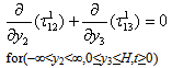(1.5)

Similarly for the half space M₂

(1.6)

Now differentiating partially (1) With respect to y₂, (2) with respect to y₃ and adding and using (5) we get,∇² u₁ = 0 for

(1.7)

(1.8)

We have the following boundary conditions:

Boundary Conditions on Stress

Continuity in stress condition:

(1.9)

(1.10),

(1.11)

Where, τ∞ (t) is the tectonic force which arise due to convection current acting at a far distance from the fault and always keeps the layer in a stressed state.

Boundary Conditions on displacement

As we have assumed the layer and half space are in welded contact.

The displacement is continuous.

(1.11.1)

Initial Conditions:

(1.12)

Taking Laplace transformation from (7) to (11a)

(1.13)

(1.14)

(1.15)

We are to solve the boundary value problem (1.12) to (1.15)

3. Solutions in Absence of Fault Creep ([24], [25])

Solving the boundary value problem, (1.12)-(1.15)

We get,

(2.1)

(2.1.1)

(2.1.2)

If we take τ∞(t) = constant = τ∞ (say)

Then,

(2.2)

(2.3)

(2.4)

If we take τ∞ = 200 bars = 200 x 10⁶ dynes/cm² and η₁ = 10²¹ poise then, = 2x10−¹³ /sec = 6 x 10−⁶ / year which tally with the observational value which is order 10−⁶ to 10−⁷.

4. Displacements and Stresses after the Commencement of Fault Creep across the Fault F₁:([24],[25])

In our paper we are considering 1 creeping fault in the layer M₁.

If the creep commences across F at time t = T₁, then the relations (1.1) to (1.10) are satisfied and we have the following creeping conditions.

(3.1)

Where F is the fault located in the region y₂ = 0, and 0 < y₃ < D₁ and t₁ = t − T₁,

is the discontinuity in the displacement u₁ across the fault F₁.

(3.1.2)

∴ = 0 for t₁ < 0 and H (t₁) Heaviside unit step function.

∴ The velocity of the creep is

where

Taking Laplace transformation of (3.1)

(3.2)

where is the Laplace transformation of u₁ (t₁) with respect to t₁ and is given by

Now we try to find u₁, τ₁₂¹, τ₁₃¹ in the form,

(3.3)

where (u₁)₁, (τ₁₂¹)₁, (τ₁₃¹)₁ are continuous every where and are therefore given by (2.1), (2.1.1), (2.1.27).

We are only to find (u₁)₂, (τ₁₂¹)₂, (τ₁₃¹)₂ which depend on the fault creep across F₁. The values of (u₁)₂, (τ₁₂¹)₂, (τ₁₃¹)₂ are assumed to be zero for t < T₁.

We have the new constitutive equations

(3.4)

(3.5)

Now stress equation of motion

(3.6)

Proceeding as before, we get,

(3.7)

New set of boundary conditions

(3.8)

(3.9)

We are to solve (3.7) – (3.9)

We take Laplace Transformation of (3.7) – (3.9)

(3.10),

(‾τ₁₃¹ )₂ = 0 on y₃ = H(−∞ < y₂ < ∞, t₁>0),

(3.11)

We shall solve (3.7) to (3.11) with the creep condition (3.1), (3.2) by modified Green’s function technique by ([9]),([21]), to get

(‾u₁ )₂ and then using

(3.12)

(3.13)

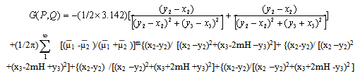
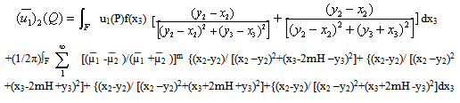
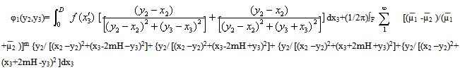
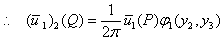
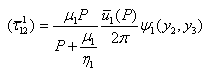
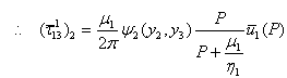
We shall get , finally, inverse Laplace Transform of which will give (u₁)₂ (τ₁₂¹)₂, (τ₁₃¹)₂.

Now let Q (y₁, y₂, y₃) be any point in the M₁ and P (x, x₂, x₃) be any point on F₁. The by ([9]),

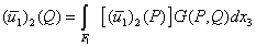(3.14)

where G (P, Q) is the G.F. and

is the discontinuity in

across F₁ and is given by

where P= Laplace transformation variable.

Therefore, from we get,

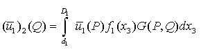(3.15)

where the Green’s function,

G(P,Q)= (∂/∂x₂) G₁(P,Q)

where,

(3.16)

(3.17)

Thus we have,

(3.18)

where f (x₃) = creep function.

On the fault F₁, x₂ = 0

Let,

(3.19)

Therefore we get,

On the fault F₁, x₂ = 0

(3.21)

Similarly we get,

(3.22)

On the fault ,x₂ = 0

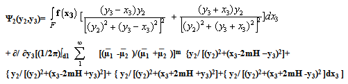(3.23)

Taking Laplace transformation we get,

(3.24)

(3.25)

(3.26)

where, a=(µ₁/ µ₂)-1,b=(µ₁/ µ₂)+1, a₁=(µ₁/ b)[(1/ µ₁)+ (1/ µ₂)]

b₁=(µ₁ µ₂ / µ₁²- µ₂²)[( µ_2/η₂)- ( µ_1/η₁)] ,a₃= a₁ -( µ₁/η₁)

T_r(t)= e^-(µ₁/η₁^)t[1- e^a₃^t e_r-1(a₃t)],

where,

e_r-1(a₃t) =1+(a₃t)+(a₃t)²/2+.....................+( a₃t)^r-1/(r-1)!

r-1>=0,e₀(a₃t)=1. (A)

5. Numerical Computations

Following [1] and recent studies on rheological behavior of crust and upper mantle by ([4], [7]) the values of the model parameters are taken as :

µ₁=3.10¹¹dynes/cm²,µ₂=2.10¹¹ dynes/cm² ,η₁= 2.10²¹ poise and η₂=3. 10²¹ poise .

D₁ = Depth of the fault = 40 km., [nothing that the depth of all major earthquake faults is in between 10-35 km].

=constant= dynes/cm² (200 bars), [post seismic observations reveal that in most of the cases, stress released in major earthquake are of the order of 200 bars or less, in extreme cases, it may be 400 bars.]

₁₂(y₂,y₃,0)= 5x10⁷dyne/cm² (50 bars),and

We take the creep function, ,with U=1cm/year, satisfying the conditions stated in .

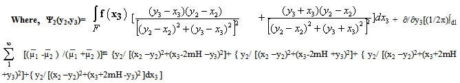
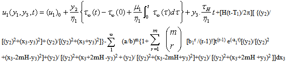
The rate of change of shear strain is:

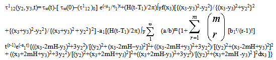
∂/∂t(e₁₂¹)=1_/η₁+(τ_H/η₁)y₃+[(H(t-T)/2π)∫_F [(a/b)^m{1+ [b₁^r/(r-1)!][-a₁t^(r-1)e^(-a₁^t)+(r-1)t^r-2

e^(-a₁^t)]{((x₃-2mH-y₃)²-3y₂²)/[(y₂)²+(x₃-2mH–y₃)²]²+((x₃-2mH+y₃)²+3y₂²)/[(y₂)²+(x₃-2mH+y₃)²]²+((x₃+2mH+y₃)²-3y₂²)/[(y₂)²+(x₃+2mH+y₃)²]²+((x₃+2mH-y₃)²-3y₂²)/ [(y₂)²+(x₃+2mH-y₃)²]²dx₃]} (3.27)

The rate of shear stress12 is:

[∂τ¹₁₂(y₂, y₃,t)/∂t]= ^-(µ₁/η₁⁾ [ τ_∞(0) –(τ¹₁₂)₀]e^-(µ₁/η₁^)t

+[(H(t-T₁)/2π)

∫_F (a/b)^m{1+ [b₁^r/(r-1)!][- a₁t^(r-1) e^(-a₁^t) +(r-1)t^r-2 e^(-a₁^t)]{((x₃-2mH-y₃)²+3y₂²) / [(y₂)²+(x₃-2mH –y₃)²]²+ ((x₃-2mH+y₃)² +3y₂²) / [(y₂)²+(x₃-2mH +y₃)²]²+ ((x₃+2mH+y₃)²+3y₂²) / [(y₂)²+(x₃+2mH +y₃)²]²+((x₃+2mH-y₃)²+3y₂²)/[(y₂)²+(x₃+2mH-y₃)²]²dx₃]}

(3.28)

6. Discussions and Conclusions

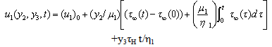
(A) Variation of displacement due to the creep movement across the fault after t₁=1year.

Equation (3.24) gives the displacement U1 at any point (y₂,y₃) at any time t, due to the fault movement across the fault F. Fig 2 shows the variation of displacement U1 with depth y₃ for y₂=8km. t=1year.It is observed that maximum displacement occurred at y₃=0 and it’s magnitude is 2.25 cm/year and it gradually decreases to zero at a depth about 100km from the free surface.

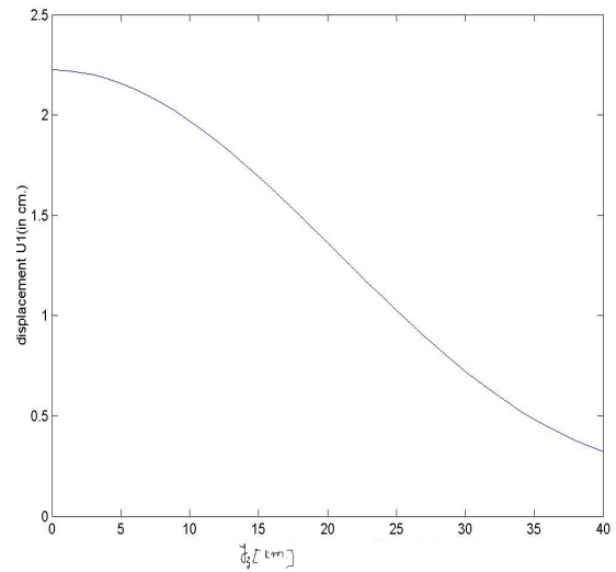Figure 2. shows the variation of displacement U1 with depth y3 for y2=8km. t1=1year due to fault movement

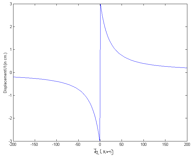Figure 3. shows the variation of surface displacement U1 for y3=0km.and t1=1year with y2 due to the fault movement across the fault F

We observe that the displacement has a discontinuity at y₂ =0km and is antisymmetric about the fault plane.

(B) Rate of change of surface displacement before fault movement.

Equation (3.24) gives the displacement u₁ at any point (y₂, y3) at any time t, before the fault movement across the fault F. We have ∂u₁/∂t=y₂/η₁ which represents a straight line through the origin with slope <<1.

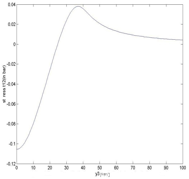Figure 4. shows the variation of stress t12 with y3 for y2=5km.t1=1year due to the fault movement across the fault F

(C) Variation of stress 12(t₁₂ , which is the main driving force) due to the creep movement across the fault after t₁=1year.

Equation (3.25) gives the stress component 12 at any point (y₂,y₃) at any time t, due to the fault movement across the fault F.

Fig 4 shows the variation of stress t₁₂ with y₃ for y₂=5km.t=1year due to the fault movement across the fault F. We observe that stress 12 releases up to a depth about 20km. and then begin to accumulate. The maximum accumulation occurred at a depth about 40km with a magnitude of about 0.39 bar per year but the rate of accumulation gradually decreases to zero at a depth of about 150km.

(D) Variation of shear stress t₁₂ with time ‘t’.

Equation (3.28) gives the rate of change of shear stress t_{12 .} Fig 5 shows the variation of stress t₁₂ with time ‘t’. It is observed that the graph is a straight line parallel to time axis, i.e. the rate of change of shear stress is constant.

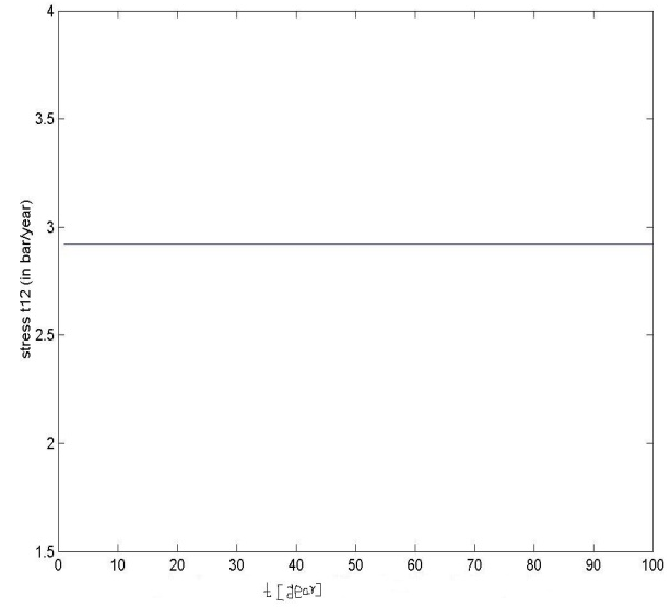Figure 5. variation of shear stress t12 with time ‘t’ for y2=5km. y3=10km

(E) Variation of surface shear strain E₁₂ (say) for t₁=1 year for y₃=0km. with y₂ due to the fault movement.

Equation (3.26) gives the variation of surface shear strain E_{12 .}Fig 6 shows the variation of surface shear strain E₁₂ with y₂ for y₃=0km and t=1 year due to the fault movement. It is observed that the surface shear strain is maximum near y₂=0, it’s magnitude is 2*10^-6 and gradually decreases as we go away from the fault.

(F)Rate of change of surface shear strain:

Equation (3.27) gives the rate of change of shear strain e_{12 .} Fig 7 shows the variation of stress e₁₂ with time‘t’. It is observed that the graph is a straight line through the origin and it’s magnitude is of order 10^-6 which well matched with the observational data.

[U1 is the component of displacement, t₁₂ is stress component and E₁₂ is the component of shear strain due to the fault movement]

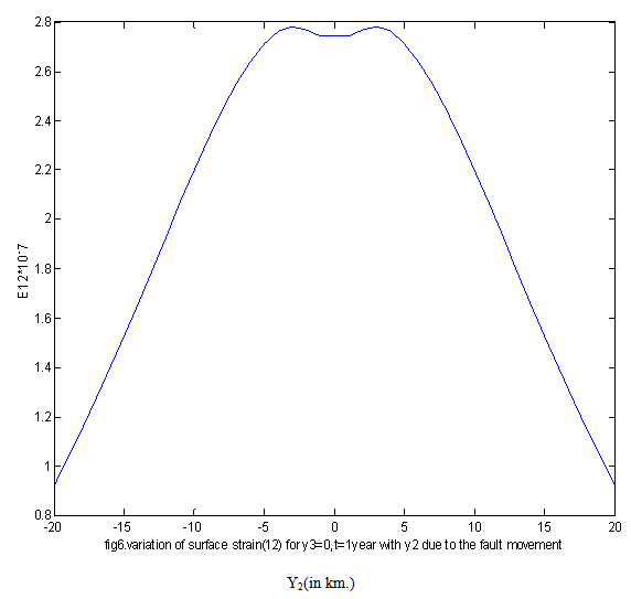Figure 6. variation of surface shear strain E12 for t1=1 year, with y2 for y3=0km.due to the fault movement

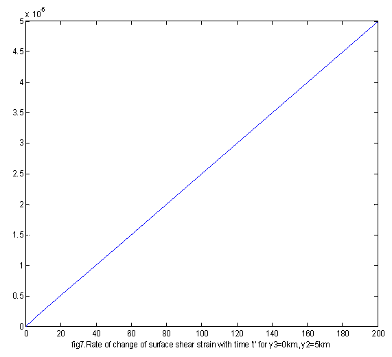Figure 7. Rate of change of surface shear strain e 12 for y3=0,y2=5km

ACKNOWLEDGEMENTS

One of the authors (Subrata Kr. Debnath) thanks the Principal and Head of the Department of Basic Science and Humanities, Meghnad Saha Institute of Technology, a unit of Techno India Group(INDIA),for allowing me to pursue the Ph.D.thesis, and also thanks the Geological Survey of India, Kolkata, ISI Kolkata, for providing me the library facilities.