1. Introduction

Alaska area, which is located on the North East of Pacific Ocean Ring of Fire, is an area of tectonic in front zone of plate collision between the Pacific plate and the North American continent plate in the form of subducting Ocean plate below the continental plate.

According to Ref.[1], at subduction areas in Alaska, due to the collisions between continental and ocean plates, the structure of the soil that experience compression (side Ocean plate) will show positive speed anomalies. On the contrary, observed velocity of the continental shelf area shows negative anomalies. This kind of velocity structure is obtained by inverting P wave travel time data [2—4]. This research interprets S velocity structure, which is obtained from the shear wave, in the front zone of the same subduction zone through seismogram analysis in time domain and three components of ground movement.

Quantitative analysis that can be performed on a seismogram is measuring the arrival time of wave phases and dispersion analysis on surface waves.

The most easily obtainable data is P wave arrival time, because it is the first break. Ref.[1] use P wave arrival time data in their research. S waves arrival time on a station with small epicenter distance is more difficult to measure, because it has longer period and not a first-breaks and is located in a noisy environment.

The standard isotropic Earth Models PREM[5] and IASP91[6], are often used as a reference in the regional seismological research as an initial Earth model. Most seismologists have interpret the model Earth in this research area (Alaska) using travel time data and Rayleigh wave dispersion data only based on one component z[7],[4], [8—11].

In this study the Earth model in front of subduction zone in Alaska was examined through seismogram comparison of 12/30/1995, coded using old CMT format as B123095A earthquake which hypocenter is located in Alaska subduction zone, in the time domain, the waveform of S, Love and Rayleigh surface waves will be observed. The Earth model obtained by processing travel time data was retested whether it can result synthetic seismogram which resembles the observed one. The entirety of the information contained in the seismogram was used to test the Earth models.

2. Research Methodology

The earthquakes analysed in this study took place in the centre of Alaska, USA. Seismogram Data is obtained from Databank Centre (see http://dmc.iris.washington.edu), where data is accessed through the webpage. Earthquake produces ground movement, which is recorded by a station in the direction of the three local Cartesian components (North-South, East-West and Z vertical), in the receiving station.

The observational stations are located at DGR, DPC, COR and ERM. The ground movement is a complex 3-dimensional space. To alter the components of the ground movement into P-SV and SH wave, then the horizontal plane formed by the local N-S and E-W axes at receiving stations must be rotated, such that local 'North' of the observation station is directed at small arc from the observation station to the earthquake epicentre (back-azimuth). Redirection is required to satisfy the wave propagation theorem, that the complex ground movement can be described into P-SV wave in z, r and SH components in the t component.

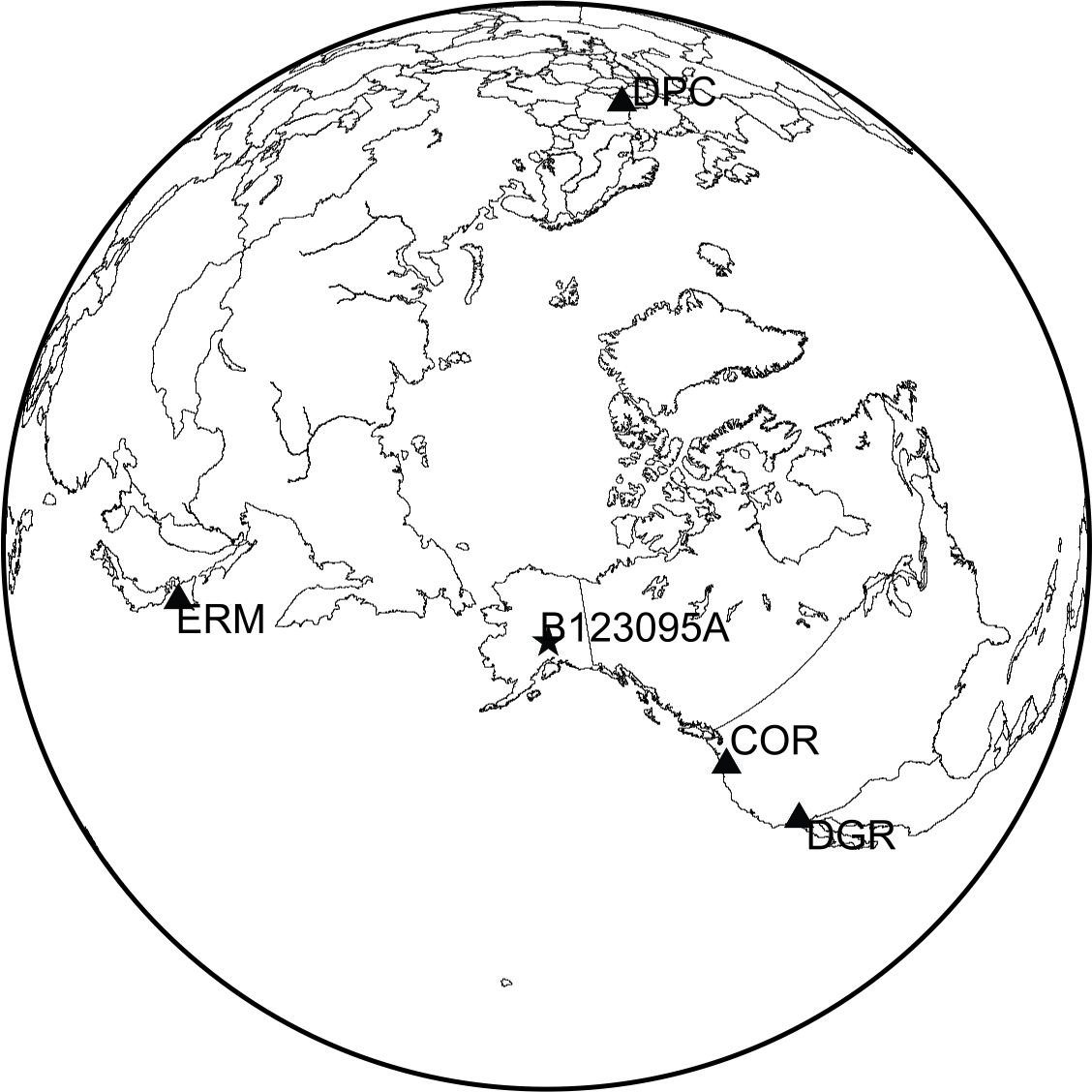
Figure 1. The locations of DGR, DPC, COR, ERM observation stations and earthquake epicenter

In this study, the first step is to run a computer program to calculate the travel time of the main body waves, the P and S wave and their repetitions. The TTIMES Program[12] is retrieved from http://orfeus.knmi.nl. TTIMES Program can only calculate travel time of synthetic body waves, it can’t calculate the surface’s wave travel time. The amplitude of the body wave decays to the inverse of distance, while surface waves have greater amplitude, because the amplitude only decays as the inverse of the root square of distance. Therefore, at a great epicenter distance, the amplitude of body also decays greatly. Surface waves propagate horizontally along the Earth surface to a depth that is ‘equal’ to the wavelength[13]. Surface waves travel time cannot be calculated, but is clearly visible in the seismogram, with larger amplitude, long oscillation and arrived after S wave. GEMINI Program[14-15] used to produce a complete synthetic seismogram, including body waves and surface waves, also core reflected wave. When this program is executed, an Earth model has to be given as an input. As input, data must contain complete elastic parameters, i.e. propagation velocity of P and S waves of rocks that constitutes the Earth's structure, mass density, quality factor and also vertical anisotropy[16]. PREM Earth model is mostly formed from P wave time travel data phase and a small portion of S wave travel time data, so that the elastic parameters obtained is P wave velocity which is more accurate and the S wave velocity which is less accurate. The other elastic parameters (mass density, anisotropy, damping factor µ and  on PREMAN Earth model obtained by inverting seismogram through dispersion analysis and method of normal model. In addition to data about the Earth's model, information is also needed on the position of the hypocenter, the moment tensor and energy released by the earthquake. All the details can be seen in the CMT catalog solution [17].

In order to compare the observed and synthetic seismogram, they should have same unit, so the response files of observed seismogram, which obtained from the requested seed file, are convoluted to the observed seismogram. This file contains the description of the phase and amplitude changes on the system equipment that involved in the entire process of earthquakes data recording, when the seismometer sensor changes ground movement input from mm/s into Voltage mV.

3. Discussion and Analysis

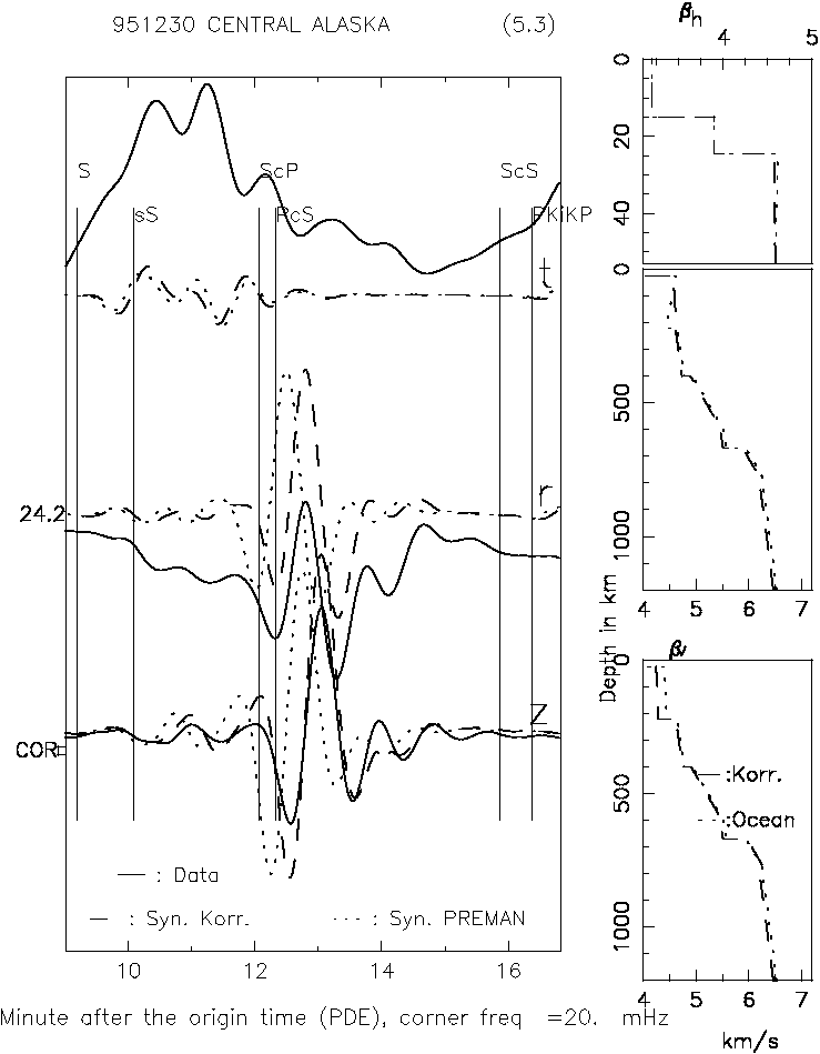
Figure 2. Seismogram analysis and fitting of B123095A earthquake at COR station

Figure 2 presents the seismogram analysis and fittings of B123095A earthquake at COR observation station, which is located South-East of the epicenter. The dotted curve reveals synthetic seismogram that is calculated from PREMAN Earth model, observed from z and r components with large amplitude is Rayleigh surface waves. Synthetic seismogram from PREMAN gives Rayleigh wave which arrived earlier than the observed Rayleigh. A well fitting is provided by synthetic seismogram from corrected Earth model on this Rayleigh surface wave phase. We can see a nice fitting which is also obtained on several phases of body wave, with smaller wave amplitude located earlier than the Rayleigh waves. Fitting is obtained by adding small value on zero-order coefficients on the velocity function in the Earth layers, from the Earth's crust down to mantle layers.

Figure 3a displays seismogram analysis and fitting on observation station DPC, which is located North-East from B123095A earthquake epicenter. If we can only analyze the components of the P-SV wave, which are Rayleigh wave and several body wave phases on COR station. Contrary, on DPC station we can clearly see the transversal component, i.e. SSH and Love surface waves, with a large amplitude. PREMAN synthetic seismogram provides Love wave with 5 wave maximum, indeed the first maximum located near the observed one, but the next maximums PREMAN synthetic Love waves arrive later than the observed maximum waves. To obtain a good fitting on the first, third and further maximums of the Love wave, the velocity gradient in the upper mantle is converted from negative, as stated in PREM anisotropic Earth model, into positive values, and then it compared with negative gradient on the PREMAN Earth model, and also by altering the values of the zero-order coefficients on the velocity structure coefficients β from upper mantle until Earth mantle below. Changes of coefficients value are required in order to obtain great fitting on the SSH body wave. Figure 3b displays that seismogram fitting is also obtained on wave S. To obtain the fitting on the S wave, S velocity change is implemented on earth mantle layers until a depth of 670 km. This means, negative anomalies in the structure of the velocity also happens to this depth, not only occur in the upper mantle.

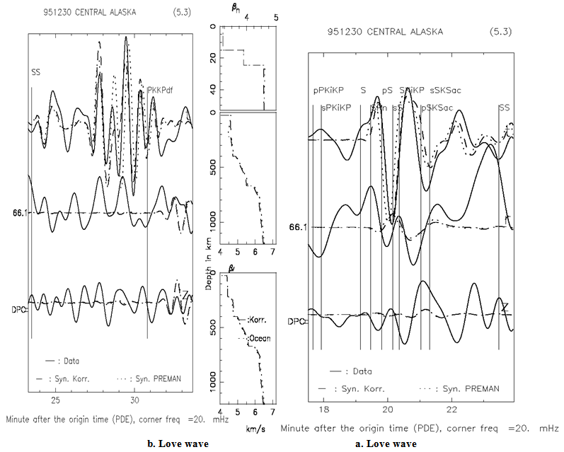
Figure 3. Seismogram analysis and fitting of B123095A earthquake on DPC station, time window a. surface wave and b. S wave

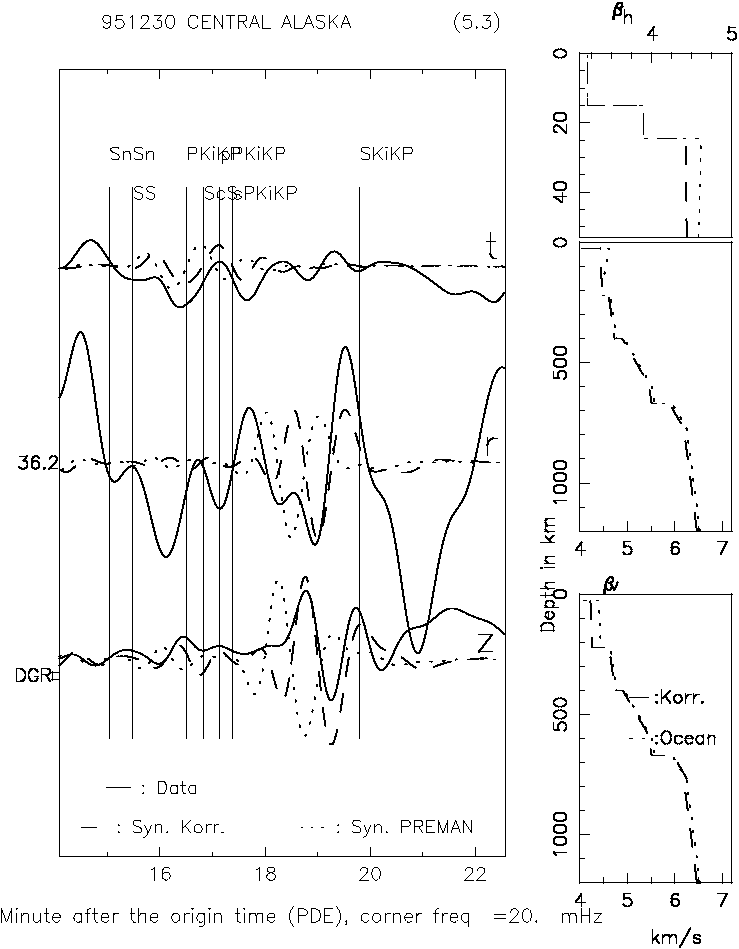
Figure 4. Seismogram analysis and fitting of B123095A earthquake on DGR station

Figure 4 presents seismogram comparison on DGR observation station. PREMAN earth model provides Love wave that arrives earlier than observed Love wave. This means the velocity correction β_h is negatives in the upper mantle. Correction on the velocity structure β_v in the upper mantle is also negative, to get the fitting on the Rayleigh wave. A good Fitting can also be obtained on the SS wave, see trace z on 16’ minutes. This indicates that the S negative anomaly also occurs until depth of 670 km.

Figure 5 shows seismogram fitting on ERM stations on the vertical movement of z component, because the data on the two other components of the seismogram, which is radial and transversal (each notation is r and t) gives very bad measured signal, swayed, so for signal range that is supposed to be idle, it gives a huge turn-off. To obtain this fitting, velocity structure β in the upper mantle must be reduced, because Rayleigh synthetic wave from PREMAN arrived earlier. Velocity correction must also be implemented in deeper layers, although only smaller correction factor, because S phase from PREMAN still come earlier than the observed S wave.

Seismogram comparison on COR, DGR and ERM stations, where all three are located in front of the subduction zone stated that the S velocity structure in this area also have negative velocity anomalies, such as negative anomaly on P velocity which is the[1] research conclusion.

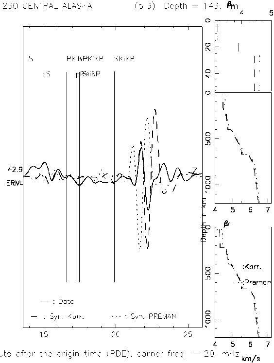
Figure 5. Seismogram analysis and fitting of B123095A earthquake on ERM station

4. Conclusions

This research carries out seismogram analysis in time domain and the three Cartesian components simultaneously, to obtain more complete information in the seismogram, compared to the analysis using only wave phase travel time and analysis of dispersion.

Simulation and comparison of seismogram can only be made up to 20 mHz frequency, because significant discrepancies has been observed on surface waves and S waves. At higher frequencies, e.g. with corner frequency of 45 mHz, strong discrepancies in the waveform shows Earth model that deviates from the supposed model.

On 20 mHz corner frequency, surface waves propagate to a depth equal to the upper mantle, thus fitting can be obtained by changing the velocity structure until upper mantle layer, where changes are made on a velocity gradient with respect to depth. Changes in the upper mantle structure did not bring improvements to the S wave phase. Further correction was carried out on the shear wave velocity propagation structure on deeper Earth layers, until a good fitting obtained on S wave. Results of this research show that the S velocity structure in front zone of the subduction zone in Alaska subsurface also has negative anomalies, such as P velocity anomaly.

References

[1]  Engdahl, E.R. and Gubbins, D., Simultaneous travel time inversion for earthquake location and subduction zone-structure in the Central Aleutian Islands, Journ. Geophys. Research, 92 (1987), B1, 13.855 -- 13.862
[2]  Cheng Qi, Dapeng Zhao, Yong Chen, Natalia A. Ruppert, 2007. New insight into the crust and upper mantle structure under Alaska, Polar Science 1, 85 – 100.
[3]  Jolly, A.D., Moran, S.C., McNutt, S.R., Stone, D.B. 2007. Three-dimensional P-wave velocity structure derived from local earthquakes at the Katmai group of volcanoes, Alaska. Journal of Volcanology and Geothermal Research 159, 326–342
[4]  Zhao, D., 2004. Global tomographic images of mantle plumes and subducting slabs: insight into deep Earth dynamics. Phys. Earth Planet. Int. 146, 3–34.
[5]  Dziewonski, A.M. and Anderson, D.L., Preliminary reference Earth model, Phys. of the Earth and Plan. Int., 25 (1981), 297 – 356
[6]  Kennett, B.L.N. Engdahl, E.R. and Buland R., 1995. Constraints on seismic velocities in the Earth from travel times, Geophys J Int, 122, 108 – 124.
[7]  Zhao, D., Christinsen, D. and Pulpans, H., 1995, Tomographic imaging of the Alaska subduction zone, Jour. Geophy. Res., 100, B4 , 6487 – 6504.
[8]  Fiona A. D., 2005, Upper mantle structure of Arctic Canada from Rayleigh wave dispersion, Tectonophysics, In Press.
[9]  Ritsema, J., van Heijst, H.J., Woodhouse, J.H., 2004. Global transition zone tomography. J. Geophys. Res. 109, doi:10.1029/2003JB002610.
[10]  Vuan,A., Maurice, S.D.R., Wiens, D.A. and Panza, G.F., Crustal and upper mantle S-wave velocity structure beneath the Bransfield Strait (West Antarctica) from regional surface wave tomography, Tectonophysics, 397 (2005), 241 – 259.
[11]  Dalton, C.A., Ekström, G., Dziewonski, A.M., 2008. The global attenuation structure of the upper mantle. J. Geophys. Res., 113, http://dx.doi.org/10.1029/2007JB005429
[12]  Bulland, R. and Chapman, C., Travel time Calculation, BSSA, 73 (1983), 1271 – 1302.
[13]  Friederich W., Regionale, dreidimensionale Strukturmodelle des oberen Mantel aus der wellentheoritischen Inversion teleseismischer Oberflaechen-wellen, Berichte des Instituts fuer Geophysik der Universitaet Stuttgart, 9, 1997.
[14]  Dalkolmo, J., 1993, Synthetische Seismogramme fuer eine sphaerisch symmetrische, nichtrotierende Erde durch direkte Berechnung der Greenschen Funktion, Diplomarbeit, Inst. fuer Geophys., Uni. Stuttgart.
[15]  Friederich, W. and Dalkolmo, J., Complete synthetic seismograms for a spherically symmetric earth by a numerical computation of the green's function in the frequency domain, Geophys. J. Int., 122 (1995), 537-550.
[16]  Takeuchi, H. and Saito, M., Seismic surface waves in Computational Physics, Academic Press, 1972
[17]  Dreger, D.S., “Time-Domain Moment Tensor INVerse Code (TDMT_INVC)”, The Berkeley Seismological Laboratory (BSL), report number 8511, 2002.