1. Introduction

Water scarce countries such as South Africa are increasingly threatened by pollution and sedimentation of water bodies due to suspended sediment concentrations in streams which affects water use and ecosystem health (e.g.[1]-[5]). It is imperative to devise the means through which these problems can be controlled but prevention and remediation relies largely on the understanding of factors controlling the sediment dynamics in a catchment, including sediment generation, transport and deposition ([6],[7]).

The term connectivity is used to describe the extent to which sediment generated on hillslopes is connected to a channel by overland and subsurface flow, as well as the linkage of streamflow and sediment within a channel network ([2],[8],[9]). Connectivity aspects from hillslopes to channels, as well as channel connectivity downstream needs to be considered. Good vegetation cover usually reduces connectivity from hillslopes to channels[2], whereas different sinks reduce connectivity within channels ranging from partial retention in small wetlands[10] to full blocking in large reservoirs[9]. At the catchment-scale, connectivity aspects are driven by complex physical processes that involve interaction of a large number of spatial and temporal factors that cannot be monitored directly[4]. Spatial and temporal variability poses a severe limitation, not only for local-scale measures, but also for procedures with a lumped nature, such as sediment rating curves and sediment delivery ratios that do not take connectivity aspects into account ([11],[12]). Assessments are usually carried out by means of semi-distributed models such as the Soil and Water Assessment Tool (SWAT)[13]-[15]. Semi-distributed models such as SWAT, however, employ certain compromises or assumptions that disregard connectivity aspects[11].

In this context, the aim of the study is twofold: to apply the SWAT model in scenario analysis to assess sediment migration and associated connectivity aspects at the catchment scale, including the influence of identified source and sink zones; and to evaluate the suitability of SWAT for use in connectivity studies. This will be achieved by means of three objectives. The first objective is to model sediment migration with SWAT in a catchment (Mkabela near Wartburg, South Africa) with identified source and sink zones. Reference[16], by means of sediment fingerprinting, identified a cabbage plot in one of the upper sub-catchments as an important source of sediment, whereas farm dams and wetlands downstream function as sinks (details provided in the section below: Site description). By means of scenario analysis, the second objective is to establish the extent that sediment outputs from the identified sediment source (cabbage plot) create input for downstream sub-catchments, as well as the impact of major sinks (9 farm dams and 5 wetlands) on sediment yield downstream. The third objective is to investigate the suitability of SWAT for use in sediment migration modelling and connectivity studies by comparing model outputs with the sediment fingerprinting study of[16]. To our knowledge, previous studies have not applied and critiqued the SWAT model within context of connectivity. Our study provides insight into the applicability of SWAT in connectivity studies, specifically describing key strengths and weaknesses of the model when assessing sediment migration and catchment connectivity. Other implications of the study include supplementing the limited number of catchment-scale connectivity studies in general, as well as incorporation of small sediment sinks including farm dams and wetlands in catchment-scale modelling, an aspect neglected particularly in dryland agricultural regions, such as in South Africa. Although connectivity largely depends on rainfall duration and intensity to produce connected flow or transport of sediment[4], SWAT is not designed as a field-scale event-based model. Therefore, the emphasis herein is on annual average results on sediment migration as represented by the SWAT model’s spatial elements including sub-catchments and catchment. Our discussion focuses on a spatial scale beyond the variability of infiltration and we do not consider the influence of subsurface flow on connectivity due to the lack of appropriate data.

2. Materials and Methods

2.1. Site Description

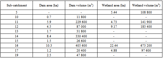
The Mkabela catchment lies between 29º 21' 12'' and 29º 27' 16'' south and 30º 36' 20'' and 30º 41' 46'' east in the KwaZulu-Natal Province of South Africa, northeast of the town Pietermaritzburg (see Figure 1). Elevation ranges from 880 m at the catchment outlet in the southwest to 1 057 m upstream in the northeast of the catchment. The catchment area of 4 154 ha is drained by a tributary of the Mgeni River with a flow length of approximately 12.6 km from its source to the catchment outlet. Connectivity is influenced by a series of 9 farm dams and 5 wetlands along the axial valley, ranging between 0.6-10 and 5.4-22 ha, respectively (see Table 1 and Figure 2 in the Model input section). Landforms are complex, ranging from gently undulating footslopes and valley floors to very steep midslopes exceeding 20%. The climate is sub-humid with a mean annual rainfall of 825 mm of which around 80% is recorded in the summer season extending from October to April. The mean annual potential evaporation is 680 mm, as estimated by the Priestley and Taylor method[17] in SWAT. July is the coolest month whereas February is the warmest month with mean minimum and maximum temperatures ranging from 6 to 21ºC and 17 to 28ºC, respectively.

Figure 1. Location of Mkabela catchment in the KwaZulu-Natal Province, South Africa

The geology consists of sandstone of the Natal Group of the Cambrian Age and a relatively small pocket of Ecca sedimentary rocks in the north[18]. Soils vary from poorly drained clays predominately in the northern part of the catchment and areas with low relief (e.g. Westleigh form) to well drained sandy soils mainly in the southern part of the catchment in areas with high relief and steep slopes (e.g. Hutton form)[19]. The major soil types occur in the central part of the catchment, including shallow sandy soils on steep and convex hillslopes with little water holding capacity (Cartef form occupying approximately 36% of the catchment) and deeper sandy soils on midslopes with soft or hard plinthic sub-horizons that is permeable to water (Glencoe and Avalon forms occupying approximately 20% of the catchment). The catchment falls within the Savanna Biome[20] but natural vegetation in the catchment has been replaced or modified by agricultural activities several decades ago. Most of the catchment is under sugarcane cultivation (3 100 ha or 75% of the catchment) with minority land uses including forestry (13%), pasture (8%) and a cabbage plot (3%) (see Figure 3a in the Model input section). Reference[16], by means of sediment fingerprinting, identified the cabbage plot in sub-catchment 1 as an important source of sediment, whereas farm dams and wetlands downstream function as sinks. The wetland in sub-catchment 11 is the major sink for the cabbage sediments (Figure 2).

Figure 2. Sub-catchment boundaries, outlets, location of river channel, farm dams and wetlands

2.2. Model selection and Description

The Soil and Water Assessment Tool (SWAT) was selected mainly because it is a spatially semi-distributed model that has gained international acceptance and has been applied to support various large catchment (10–10 000 km2) modelling studies across the world with minimal or no calibration effort (e.g.[21][23]). The foundational strength of SWAT is that it considers most connectivity aspects into one simulation package, including factors controlling upland sediment generation, channel transport and deposition into sinks[14]. Furthermore, SWAT is routinely coupled with geographical information systems which, according to[24], offer unprecedented flexibility in the representation and organization of spatial data.

SWAT is a catchment-scale, continuous time model operating on a daily time-step developed by the US Department of Agriculture (USDA) Agricultural Research Service to simulate water, sediment and chemical fluxes in large catchments with varying climatic conditions, soil properties, stream channel characteristics, land use and management practices ([15],[25]). First, a catchment is divided into multiple sub-catchments, which can be further divided into hydrological response units (HRUs) consisting of homogeneous soil and land use characteristics[14]. The hydrologic component is based on the water balance equation in the soil profile integrating several processes, including surface runoff volume using the Green and Ampt infiltration method[26] or the USDA SCS curve number method[27]. Here, the SCS curve number method was chosen which is empirically based and relates runoff potential to land use and soil characteristics. Peak runoff rate is estimated with a modification of the rational method, where runoff rate is a function of daily surface runoff volume and a proportion of rainfall occurring until all of the catchment is contributing to flow at the outlet, known as the time of concentration[28]. The time of concentration is estimated using Manning’s Formula considering both overland and channel flow. Sediment yield caused by rainfall and runoff is computed with the Modified Universal Soil Loss Equation (MUSLE)[29], using surface runoff and peak flow rate together with the widely used USLE[30] factors including soil erodibility, slope length and steepness, crop cover management and erosion control practice. Certain nutrients and pesticides are also simulated by SWAT, but are outside the scope of this research and are not described here.

Once the loadings of water and sediment have been determined, they are summed to the sub-catchment level and routed through the stream network of the catchment including ponds, wetlands, depressional areas, and/or reservoirs[28]. SWAT incorporates a simple mass balance model to simulate the transport of sediment into and out of water bodies, where settling is calculated as a function of concentration and transportation out of a farm dam is a function of the final concentration[28]. Flow is routed through the channel using either the variable-rate storage method[31] or the Muskingum method[32], which are both variations of the kinematic wave model. Here the default variable storage method was chosen. Sediment is routed by means of a simplified stream power theory where the maximum amount of sediment that can be transported, deposited or re-entrained from a channel segment is a function of the peak channel velocity[33]. The equations mentioned above and additional theoretical documentation for SWAT is given by[28]. AVSWAT-X which is a graphical user interface for SWAT and ArcView® software extension[34] was used for this study. A description of the input data requirements follows.

2.3. Model Input

The AVSWAT-X interface requires several spatial datasets including topography, drainage network, land cover, soil, climate and land management. First, topographic and drainage network data were prepared from a digital elevation model (DEM) with a grid cell resolution of 20 m[35]. Automated routines in AVSWAT-X calculated the slope and divided the catchment into sub-catchments from the DEM. Appropriate contributing source areas and sub-catchment sizes had to be established by the user as percentage area of the entire catchment, i.e. 30%. Several studies reviewed by[14] suggest setting sub-catchment areas at much smaller percentages (<5% of the catchment) to ensure accuracy of estimates, but such values are not feasible for larger catchments as simulated in this study. The number of sub-catchment links or outlets was manually adjusted, representing all the relevant tributaries of the main river into 19 sub-catchments that are comparative in size, as well as to ensure that flow monitoring points spatially overlay with sub-catchment outlet points for calibration of model simulations with field measurements. Thus, each of the 19 sub-catchments consists of a channel with unique geometric properties not shown here including slope gradient, length and width. Manning’s roughness coefficient was assigned to each segment in order to represent conditions observed in the field. Channel erosion parameters were set to default representing non-erosive channels due to the lack of data but also to eliminate channel erosion in simulations. According to observations, most sediment is generated from agricultural fields[16]. Gullies are absent in the Mkabela catchment so that the simulated sediment yields could be interpreted according to the empirical soil loss equation MUSLE used, which does not account for gully erosion.

In addition, 9 outlets were incorporated to represent outlets at the exit from 9 farm dams. AVSWAT-X also allows relatively small impoundments such as wetlands to receive loadings from a fraction of the sub-catchment area where it is located. Figure 2 illustrates the geographical distribution and extent of the farm dams and wetlands digitized from SPOT 5 panchromatic sharpened images at 2.5 m resolution acquired in 2006, whereas Table 1 contains parameter information obtained from[36]. The discretisation resulted in the definition of 19 sub-catchments that are joined by outlets and tributary channels branching off the main channel, including 9 farm dams and 5 wetlands along the axial valley.

Table 1. Parameter information used to model each of the farm dams and wetlands in Mkabela catchment (adapted from[36])

Next, a land cover map was digitized from SPOT 5 imagery acquired in 2006, followed by ground truthing (see Figure 3a). The land cover map was linked to a database in AVSWAT-X consisting of several plant growth parameters. The plant growth component of SWAT is a simplified version of the EPIC plant growth model[37], where phenological plant development is based on daily accumulated heat units developed by[38]34]and biomass is inhibited by temperature, water or nutrient stress. SWAT also requires information on soil properties that govern the movement of water through the soil profile. An unpublished pedological soil map at a scale of 1:100 000 with textural profile descriptions for all major soils was used[39] (see Figure 3b).

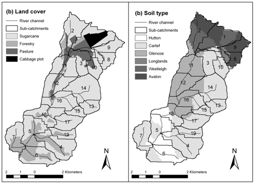Figure 3. (a) Land cover map and (b) soil map of Mkabela catchment (after[39])

In order to improve the display and representation of the variable soils in the catchment, the major soil units were delineated into smaller terrain units by means of the topographical algorithms of[40] and[41]. To account for soil variability with depth, up to three layers/horizons were incorporated into each soil component. Textural parameter values were assigned to each unit and layer according to the textural profile descriptions given by the soil map. Pedotransfer functions similar to[42] were used to generate the required hydraulic parameters, including available water capacity and saturated hydraulic conductivity. The overlay of land cover and soil maps created 130 hydrological response units (HRUs). These are portions of a sub-catchment that possess unique land use and soil attributes. Similar to[43], the discretisation was done to keep the number of HRUs down to a reasonable number, while considering the diversity and sensitivity of land cover and soil combinations. The study aimed at integrating all land cover units that significantly affect the sediment yield of a catchment, whether large or small in spatial extent.

AVSWAT-X also requires spatial data for several climate parameters including precipitation, temperature, solar radiation, relative humidity and wind speed. These were calculated from daily values over a 30 year period (1 January 1977 to 30 June 2008) from 4 stations within 2 kilometres or less of the catchment boundary[44]. Since not all the stations have full records of the required parameters, incomplete records were patched with the most complete and closest stations. Finally, ancillary information regarding management practices in the catchment was incorporated including tillage operations, nutrient applications, irrigation scheduling and harvesting operations. Due to the lack of data on crop rotation systems and timing of agricultural operations, phenological plant development is based on daily accumulated heat units. Detailed descriptions of the parameters are provided by[28].

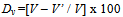
2.4. Model Calibration and Validation

Calibration and validation were restricted to measurements from an ISCO sampler and H-flume at the outlet of sub-catchment 8 (area of 96 ha) from August 2006 to March 2008, including sediment loads of 5 rainfall events between October 2007 to January 2008. Calibration of SWAT focused mainly on the hydrological part of the model on a monthly time-step adjusting the most sensitive model parameters similar to other studies (e.g.[3],[43]). The hydrological component was calibrated by modifying the curve number and base-flow coefficients, whereas the erosion component was calibrated by adjusting the MUSLE soil erodibility and support management factors. Model performance was improved by sequentially optimizing the widely used coefficient of efficiency (E) of Nash and Sutcliffe[45], as well as the coefficient of determination (r²). As a measure of goodness-of-fit between simulated and observed loads, a simple per cent deviation method[46] was used; given as:

(1)

where, V is the measured runoff volume and V’ is the simulated volume. Dv will be zero for a perfect fit and the smaller the value the more accurate are the simulated results. Subsequently, it was possible to hydrologically calibrate the model at the flume by sufficiently tracking the average monthly trends during the simulation period. Overall, SWAT over-predicted discharge by 6.2% as determined by Dv. The goodness of fit expressed by E was 70% and r² was 82%, indicating a close relationship between the observed and simulated discharge. Figure 4 illustrates the observed and simulated discharge and sediment loads of 5 rainfall events that occurred during October 2007 to January 2008. Although the limited number of observed events cannot be used to fully validate the model, there is good indication that a large part of the suspended sediment load can be explained by event discharge and that the model is able to track the loads of these events at least within the order of magnitude of observed values.

The observed data were inadequate to validate total discharge and sediment yield at the catchment outlet. Unfortunately, a major limitation to the use of continuous time models such as SWAT in developing countries is the lack of recorded flow and sediment data for calibration and validation[47]. Nevertheless, similar to the study of[43], calibrated values for specific HRUs in sub-catchment 8 were extended downstream to the larger catchment area with corresponding HRUs under sugarcane cultivation. More detail on these HRUs is outside the scope of the text. Although accurate predictions were not the goal of this study, the calibration, together with above-mentioned fingerprinting study of[16], served to establish a realistic baseline for spatially extending the AVSWAT-X model downstream in order to investigate connectivity aspects of sediment migration modelling.

Figure 4. Observed and simulated discharge and sediment loads of 5 rainfall events that occurred from October 2007 to January 2008

2.5. Connectivity Aspects in Sediment Migration

Central to this study was the assessment of connectivity aspects in sediment migration at the catchment scale with the SWAT model. In order to create a catchment overview of sediment migration downstream and the associated connectivity aspects, the study performed four additional simulations with the AVSWAT-X model after simulating the observed catchment condition with all dams and wetlands in place. Two scenarios were performed to establish the extent that sediment outputs from the identified sediment source (cabbage plot) create input in addition to sugarcane for downstream sub-catchments, whereas another two scenarios were performed to establish the impact of existing sinks (9 farm dams and 5 wetlands) on connectivity downstream. In total, 5 simulations were conducted over a period of 2 years (1 July 2005 to 30 June 2008) preceded by a one-year model “warm-up” initialization period. The four scenarios are summarized as follows:

1a. Replacing the current cabbage plot with sugarcane;

1b. Replacing existing pasture and sugarcane fields in sub-catchment 1 with cabbage, subsequently expanding the current cabbage plot by approximately 300% (from 114 to 351 ha) and connecting it with the main channel;

2a. Simulating current conditions without farm dams;

2b. Simulating current conditions without wetlands.

The results for each scenario were scrutinized for changes in the simulated sediment outputs from the upper to lower sub-catchment outlets, including dams and wetlands along the main river. This was mainly achieved by investigating the annual changes in simulated discharge and sediment loads as represented by the model’s spatial elements, namely sub-catchments and catchment.

3. Results and Discussion

3.1. Sediment Dynamics in the Mkabela Catchment

Figure 5 illustrates the sediment yield in t/ha for each sub-catchment that is transported into the channel during the observation period (1 July 2006 to 30 June 2008). Results substantiate the findings of[16] that sub-catchment 1 containing the cabbage plot is a significant sediment source. Although sub-catchment 1 is characterized by flat slopes between 0 and 2%, sediment yield (1.7 t/ha) is several orders of magnitude larger than yields (0.001 t/ha) in sub-catchments downstream (e.g. 4, 5, 6 and 7) with steep slopes up to 30%. The main reason for this discrepancy is related to vegetation cover. Latter sub-catchments contain sugarcane and forestry plantations with good seasonal groundcover, whereas sub-catchment 1 contains a cabbage plot with relatively poor groundcover. Furthermore, soil under the cabbage plot consists of poorly drained clays that are more prone to runoff and erosion than the well-drained sandy soils of sub-catchments 4, 5, 6, and 7.

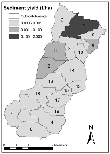Figure 5. Sediment yield per sub-catchment (in t/ha) that is transported into the channel during the observation period (1 July 2006 to 30 June 2008)

Figure 6a illustrates the monthly average streamflow in m3/s for 9 sub-catchments connected with the main channel and Figure 6b shows the total sediment in metric t per month transported out of their outlets. Streamflow ranges between 0.003 m3/s at sub-catchment 1 in September 2007 to 0.701 m3/s at the main catchment outlet in January 2008, whereas sediment loss ranges between 0.059 t at sub-catchment 9 in September 2007 to 19.46 t at the main catchment outlet in January 2008. Model outputs substantiate several logical criteria regarding sediment dynamics that are consistent with studies in other parts of the world. First, Figure 6a and 6b follow the same pattern which indicates that sediment output is controlled by the water flux. Second, results clearly illustrate a summer dominant erosion pattern which is mainly caused by intensive summer rainfall totalling 620 mm between October and April. According to simulations, nearly 70% of the average annual streamflow and over 85% of the annual sediment output (approximately 70 metric t per annum) are concentrated in the rainy season. Third, low outputs occur mainly in the upper sub-catchments and increase downstream due to the cumulative contribution of runoff and sediment routed downstream from sub-catchment outlet 8 to 7. The migration of sediment downstream explains why certain sub-catchments with relatively low sediment yields (see Figure 5) have high sediment outputs at their outlets (see Figure 6b) and vice versa. The following section discusses the impacts of identified source and sink zones on connectivity as simulated by SWAT.

3.2. Scenarios Assessing the Influence of Identified Source and Sink Zones

Scenario impacts on discharge and sediment output for 9 sub-catchments along the main channel are illustrated in Figure 7. Scenarios 1a and 1b illustrate the extent that sediment outputs from the identified sediment source (cabbage plot) create input in addition to sugarcane for downstream sub-catchments, whereas scenarios 2a and 2b establish the impact of existing sinks (9 farm dams and 5 wetlands) on connectivity downstream. Impacts are expressed as the percentage difference between current conditions and four scenarios assessing the influence of the identified source and sink zones.

3.2.1. Scenario 1a: Replacement of Cabbage Plot with Sugarcane

Replacement of the cabbage plot with sugarcane illustrates the extent that sediment outputs from the cabbage plot create input in addition to sugarcane for downstream sub-catchments. Figure 7 illustrates that replacement of the cabbage plot with sugarcane decreases average annual discharge and sediment output the most at the outlet of sub-catchment 1 containing the cabbage plot (-2.2% and -18.4% respectively) and reduces downstream (to -0.4% and -0.2% respectively at the main catchment outlet). Results indicate that the cabbage plot increases discharge and sediment output the most at sub-catchment 1 in which it is located and impact on discharge and sediment output diminishes downstream to nearly zero percent past sub-catchment 11. During the simulation period, sediment from the cabbage plot is deposited downstream mainly in the channel along sub-catchments 1, 3 and 11 (approximately 287.6 t/yr). Reasons for deposition in the channel include its relatively rough surface conditions (Manning’s roughness coefficient of 0.1), as well as the limited number of large rainfall events and associated peak channel velocities needed to transport and re-entrain sediment during the simulation period. Sediment from the cabbage plot that is not deposited in the channel is deposited in the farm dam of sub-catchment 11 (approximately 7.4 t/yr). The following scenario illustrates the effect of a larger cabbage plot on annual changes in simulated discharge and sediment loads.

Figure 6. (a) Monthly average streamflow (m3/s) for 9 sub-catchments connected with the main channel; (b) Total sediment (metric t per month) transported out of the 9 sub-catchments. Sub-catchment numbers are assigned arbitrarily

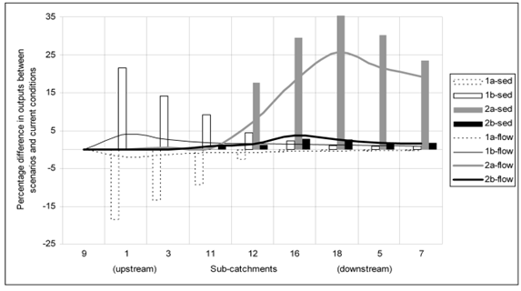Figure 7. Scenario impacts on discharge and sediment output for 9 sub-catchments along the main channel, expressed as the percentage difference between current conditions and four scenarios (1a - replacing cabbage plot with sugarcane; 1b – expanding cabbage plot by approximately 300%; 2a - current conditions without farm dams; 2b - current conditions without wetlands)

3.2.2. Scenario 1b: Cabbage Plot Expanded

In Scenario 1b, the cabbage plot is expanded approximately 300% so that it covers the whole of sub-catchment 1 at the expense of sugarcane and pasture. As expected, Figure 7 illustrates that the average annual discharge and sediment output increase the most at the outlet of sub-catchment 1 (4.0% and 21.6% respectively) and reduces downstream (to 0.8% and 0.9% respectively at the main catchment outlet). Similar to scenario 1a, the impact of the larger cabbage plot on discharge and sediment output diminishes downstream due to deposition along the channel of sub-catchments 1, 3 and 11 (approximately 760.0 t/yr), including the farm dam of sub-catchment 11 (approximately 13.0 t/yr). Compared to scenario 1a, however, outputs nearly triple and more sediment migrates beyond sub-catchment 11. This is reasonable given that there is a greater supply of sediment since cabbage has less groundcover than sugarcane and pasture, but also supposedly uninterrupted connectivity between the cabbage plot and channel. The expanded hydrological response unit covers the whole sub-catchment 1 which is locationally connected to simulated channel – although this is not accounted for in SWAT and is discussed below. The following section discusses the impact of identified sink zones on connectivity as simulated by SWAT.

3.2.3. Scenario 2a: Removing Farm Dams

Figure 7 illustrates that removal of farm dams increase discharge and sediment output the most at sub-catchment outlets downstream (11 downwards) where most of the farm dams normally occur. More specifically, average annual discharge and sediment output increase the most at the outlet of sub-catchment 18 (25.6% and 36.7% respectively). Although sub-catchment 18 does not contain a farm dam within its boundaries, seven farm dams are located near and upstream of it, subsequently retaining its loadings as illustrated in Figure 7. In relation to the amount of discharge and sediment reaching the catchment outlet, 19.2% and 23.5% is retained respectively. Since nearly all sediment from the cabbage plot is deposited in sub-catchments 1, 3 and 11 before reaching farm dams downstream, sediment deposited in farm dams mainly originates from surrounding sugarcane fields. According to the simulation, average sediment deposition per farm dam equals 6.3 t/yr. Although studies elsewhere report more drastic declines in sediment retention in dams (e.g. 64% by[21]), our results seem reasonable given the fact that the farm dams are relatively small with an average storage capacity of 136 333 m3 and regularly spill, thus frequently releasing suspended sediment[9]. Importantly, results were able to represent farm dams as a series of storages where flow is reduced, sediment deposited and thus connectivity is reduced.

3.2.4. Scenario 2b: Removing Wetlands

The impact of wetlands is investigated by simulating current conditions without wetlands. Figure 7 illustrates that removal of wetlands increase discharge and sediment output at sub-catchment outlets where most of the wetlands would occur. More specifically, average annual discharge and sediment output increase the most at the outlet of sub-catchment 16 (3.6% and 2.8% respectively) containing the largest wetland. At the catchment outlet, discharge is reduced by 1.6% and sediment output by 1.7%. Average sediment deposition per wetland equals 0.012 t/yr. Compared to current conditions without farm dams in scenario 2a, wetlands influence discharge and sediment output insignificantly, subsequently influence connectivity less than farm dams. These results remain questionable since the wetlands have a larger total area and storage capacity (47 ha and 1 204 900 m³) compared to farm dams (36 ha and 1 191 000 m³), and since the fingerprinting study of[16] established that the wetland in sub-catchment 11 is a major sink for the cabbage sediments. The following section provides a brief discussion of how model compromises or assumptions affect outputs in the context of connectivity between sources and sinks, as represented by the model’s spatial elements including sub-catchments and catchment.

3.3. Suitability of SWAT in Connectivity Studies

In terms of source zones at the sub-catchment scale, SWAT simulations substantiate the findings of[16] that the cabbage plot is an important sediment source in the Mkabela catchment (see Figure 5). Results illustrate, however, that sediment generated on the relatively small cabbage plot is not spatially identified within the sub-catchment it is located. The whole of sub-catchment 1 is highlighted as a source in Figure 5. The non-spatial aspect of hydrological response units (HRUs) ignores flow and sediment routing within a sub-catchment[14]. SWAT does not consider the processes of deposition during transport from HRUs to channel since all the eroded sediment calculated for the separate HRUs reaches the channel[11]. Comparison of the SWAT output tables of scenario 1a and current conditions not shown here indicates that all the sediment generated from the cabbage plot reaches the channel of sub-catchment 1. Likewise, the increase in percent discharge and sediment loads shown in Figure 7 for scenario 1b can be explained exclusively by the increase in the spatial extent of the cabbage plot at the expense of sugarcane and pasture, not due to its uninterrupted connectivity with the channel. In reality the potential for different HRUs of a sub-catchment to contribute to sediment yield is controlled by a complex interplay of connectivity aspects including locational and filter resistance during transport from HRUs to channel[13]. The HRU approach in SWAT disregards processes of deposition in the pasture HRUs between the cabbage plot and channel. Although filter strips and field borders can be simulated at the HRU level based on empirical functions, assessments of targeted filter strip placements or riparian buffer zones is not possible due to the lack of HRU spatial definition in SWAT[14]. Reference[24] suggests the use of smaller sub-catchments instead of HRUs, but this approach is only applicable in small catchments and the impacts on SWAT output as a function of variation in HRU and/or sub-catchments is outside the scope of the study. Reference[24] provide further detail on the extent predictions in general are altered by using HRUs, as well as the mechanisms by which sediment is moved from sub-catchments to channels.

In terms of sink zones at the catchment scale, SWAT seems to be particularly efficient in representing the farm dams as a series of storages where flow is reduced, sediment deposited and thus connectivity is reduced (see Figure 7). However, the impact of farm dams on connectivity needs further investigation in the Mkabela catchment since no measurements have been made on sediment input and output from farm dams. Results are based on the assumptions in SWAT that water bodies are completely mixed and sediment is instantaneously distributed throughout the volume at entering. SWAT could not effectively identify wetlands as sink zones and simulations do not correlate with the findings of[16] that cabbage sediment is primarily deposited in the wetland of sub-catchment 11. As mentioned above, during the simulation period of 2 years large portions of cabbage sediment is deposited in the channel along sub-catchments 1, 3 and 11 – here the channel in effect acts as a wetland due to its relatively rough surface conditions. However, not even smoother channel conditions or a longer simulation period will ensure that sediment from the cabbage plot is transported to the wetland in sub-catchment 11. Wetlands simulated by SWAT only retain the water and sediment originating from the sub-catchment within which they are located. Wetlands in SWAT cannot receive and retain loadings from the sub-catchment upstream containing the cabbage plot. In contrary to the way farm dams are simulated, wetlands are simulated off the main channel and water or sediment flowing into them must originate from the sub-catchment in which they are located[28]. This largely explains why the percentage difference in discharge and sediment output of scenario 2b without wetlands are less than that of scenario 2a without farm dams (see Figure 7). Although changing the model structure was not an objective of the study, modifications of SWAT[22] or application of other SWAT-based models such as SWIM[10] where wetland processes are incorporated more realistically may greatly improve simulation of wetland dynamics.

4. Conclusions and Recommendations

The Soil and Water Assessment Tool (SWAT) is applied within the context of connectivity in the Mkabela catchment in KwaZulu-Natal, South Africa, including the influence of identified source and sink zones. The study illustrates how the model can be applied in scenario analyses to assess connectivity aspects in sediment migration modelling. Scenario analyses establish the extent that sediment outputs from the identified sediment source (cabbage plot) create input for downstream sub-catchments, as well as the impact of major sinks (9 farm dams and 5 wetlands) on sediment yield downstream. Results are consistent with other studies where vegetation cover and soil type of source zones have major influences on sediment generation (e.g.[9],[48]), whereas structures such as farm dams serve as important sink zones where sediment is deposited (e.g.[21],[49]). More specifically, the cabbage plot is an important source of sediment because of relatively poor seasonal groundcover and poorly drained clays prone to runoff and erosion. The removal and expansion of the cabbage plot in our scenario analyses significantly changes discharge and sediment yield upstream. However, similar to the studies of[1] and[50], no significant changes are simulated at the catchment outlet. The main reason is the channel serves as an important sink zone due to its relatively rough surface conditions. Although the removal of farm dams significantly changes discharge and sediment loads at the catchment outlet, sediment deposited in farm dams mainly originates from surrounding sugarcane fields, not the cabbage plot. Subsequently, the effect of sediment sinks becomes dominant over sediment sources with increasing spatial scale as addressed by several other studies ([2],[51][53]). In order for results to be useful for site– and scale–specific management intervention, it is important to consider how model compromises or assumptions affect outputs in context of connectivity between sources and sinks, as represented by the model’s spatial elements including sub-catchments and catchment.

At the sub-catchment scale, SWAT effectively identifies the cabbage plot as an important source of sediment. However, cabbage plot sediment is not spatially identified within the sub-catchment it is located and all the sediment generated from the plot reaches the channel, whether connected to the channel or not. A major weakness of SWAT is that it does not consider the processes of deposition during transport from hillslopes/HRUs to channel[11]. Reference[24] suggests the use of smaller sub-catchments instead of HRUs, but this approach is not applicable in large catchments such as simulated here. In large catchments, discretisation should be done to keep the number of sub-catchments and HRUs down to a reasonable number, while considering the diversity and sensitivity of land cover and soil combinations. It is recommended that future SWAT-based research determine how catchment partitioning affects model outputs in the context of connectivity. Such research will require assessments at relatively fine spatial and temporal scales, including factors influencing connectivity at hillslope/HRU scale such as processes of overland/subsurface flow and site-specific process zones in channels, and relationships between different rainfall events and connectivity. Reference[7] also stresses that there is an urgent need for more emphasis on the timescale over which sediment moves through a catchment, specifically the rates of sediment movement of different sizes and from different sources.

At the catchment scale, SWAT seems to be efficient in representing the farm dams as a series of storages where connectivity is reduced. However, SWAT could not effectively identify wetlands as sink zones and simulations do not agree with the findings of[16] that sediment originating from the cabbage plot is prone to be deposited in the wetland of sub-catchment 11. In contrast to farm dams, wetlands in SWAT are simulated off the main channel and water or sediment flowing into them must originate from the sub-catchment in which they are located[28]. Therefore, it is recommended that future research in the Mkabela catchment include scenarios that account for wetland processes or impacts. For example, if the wetland is located alongside the channel the channel roughness coefficient in SWAT could be adjusted to represent wetland storage conditions. Long-term monitoring of discharge and sediment load is also recommended, including losses from evaporation and releases for irrigation in water bodies and sediment trap efficiencies.

In conclusion, SWAT results indicate the sensitivity of loads to hypothetical land use change, reflecting the spatial connectivity within the catchment due to the retention of loads mainly in the channel and farm dams. The study recommends that modellers should give sufficient attention to different connectivity aspects in sediment migration modelling, together with the way a model accounts for these aspects at different scales and from source to sink.

ACKNOWLEDGEMENTS

The authors are thankful for research funding and managerial support from the Water Research Commission, especially Mr. M. Du Plessis and the Agricultural Research Council - Institute for Soil, Climate and Water. Special thanks to Prof. A. Görgens and Ms. S. Lyons at Aurecon (formerly Nimham Shand Consulting Civil Engineers) for coordination of the larger project. The study benefited from the comments from project team members including Prof. J. Annandale, Mr. M. Van der Laan, Dr. N. Jovanovic, and Dr. B. Grové and Ms. N. Matthews. Thanks also to advice from the appointed Reference Group, especially from Prof. K.L. Bristow. The paper benefited from the comments by referees on an earlier version.