1. Introduction

1.1. Geological Setting

The San Andreas Fault defines an approximately 1300 km (800 mi) portion of the boundary between the Pacific and North American plates. Along its length, the fault undergoes horizontal strike-slip motion that accommodates most of the relative motion between the plates. To the north, a complex of transform faults and spreading centres accommodate the motion of the Gorda and Juan de Fuca plates. To the south, a similar complex of spreading centres and transform faults accommodate the displacement in the Gulf of California.

The area is situated on a relatively straight section of the San Andreas Fault in central California, where fault movement occurs as right lateral slip both in earthquakes and as aseismic slip, or "creep". From both geodetic and seismic data, currently, the southern section appears to be generating no movement or small to moderate sized earthquakes. Similarly, the section of the fault north of San Juan Bautista also has produced large earthquakes, including the 8.3 Magnitude San Francisco’s earthquake in 1906 and the 7.1 Magnitude Loma Prieta’s earthquake in 1989. Most of the northern section of the fault is also currently inactive, with with no detectable movement and few earthquakes since1906. Between these locked sections, the San Andreas Fault creeps (aseismical slip) from San Juan Bautista to Parkfield, produces numerous small (mostly M=5 and smaller) earthquakes, while no larger ones detected. The stretch of the fault between Parkfield and Gold Hill defines a transition zone between the creeping and locked behaviour of the fault.

Waveforms recorded on regional seismographs are strikingly similar with the 1922, 1934 and 1966 earthquakes, suggesting that these earthquakes caused repeated rupture in the same area on the fault. These observations suggest that there may be some predictability in the occurrence of earthquakes. In addition, much is being learned about the physics of earthquakes from advances area including the discovery of repeating micro earthquakes (see Ellsworth[1]) and earthquake "streaks" (see Waldhauser et al.[2], and Rubin et al.[3]).

A "creeping" section (green) separates locked stretches north of San Juan Bautista and south of Cholame. The Parkfield section (red) is a transition zone between the creeping and southern locked section. Stippled area marks the surface rupture in the 1857 Fort Tejon earthquake. (http://earthquake.usgs.gov/research/parkfield/geology.php)

1.2. Standard Earth Models

The knowledge of the shear wave velocity in the lithosphere and in the mantle is important for our understanding of the tectonic regime that influences the evolution of a continental region. The velocity is a strong function of temperature, more than composition, and may decrease dramatically in the presence of volatiles or melting[4].

Information about the S velocity in the lithosphere and mantle is obtained from surface wave[5,6]. There are some researches that based on the travel times method in this region[7—9], that had been applied to obtain the structure of P and S wave velocities in 1, 2 or 3-D Earth model. The structures of S wave velocity near the CMB (Core Mantle Boundary) and earth core are analysed through the travel time of SKKS waves. Such wave phase can be observed at station with epicentral distances greater than 83⁰[10,11].

Tomography method is appropriate with dispersion analysis, where the observed data measures the relation between phase/group velocities to frequencies/periods. There are various methods to measure the dispersion curve, for example Multiple Filtering Technique[12] that is phase-matched by MFT for the insulation of basal mode of surface wave[13]. Inversion is carried out with the goals to get the fitting between both velocities of observed and predicted. From this fitting a more detailed earth models is obtained, either 1-D or 3-D, for example[5,6,14—16].

Both methods to obtain the earth models are achieved by evaluating only a little information of the seismogram. This research analyses the waveform in the time domain with three components simultaneously. It will be shown how sensitive a waveform is to structure of an Earth model by covering structures of speed and anisotropy within the Earth. This research also shows at what depth the layers meet the vertical isotropy in the earth model.

This study tried to answer the following question: Are standard earth models obtained by evaluating only the travel time data and dispersion analysis could yield a synthetic seismogram with three components which is similar to the observed one, if the seismogram analysis is carried out with a corner frequency of 20 mHz[17]?

2. Method

Every earthquake yields ground movement at any station, which can record its three Cartesian component (N-S, E-W and vertical Z) known as channels with the suffix – E, – N & – Z. The location of the earthquake epicentre is in Guerrero, Mexico, at coordinates 18.68⁰ North Latitude and 101.60⁰ West Longitude. To dissociate the complex ground movement into the wave propagation of P, SV waves and SH wave, the horizontal area formed by the orientation of the local N-S and E-W at the observation station have to be rotated in such a way that the rotating angle between the local 'North' and the direction of a small arc from the station to the epicentre (back-azimuth) is reached so that the movement is decomposed into the direction of transversal and radial of ground movements.

To identify the wave phases in the seismogram, program TTIMES[18] is used to compute the travel times calculations. The calculation of synthetic seismogram is based on the GEMINI method[19,20]. When running the GEMINI program, an Earth model, either IASPEI91 or vertical anisotropic PREM (hereafter PREMAN) is given as initial input. The earth model should contain data that describes the structure, density, velocity function, quality factor, ρ, α, β, and κ.

3. Seismogram Results and Analysis

This study analyses the seismic data of earthquake that occurred in May 22^th, 1997 on Guerrero, Mexico, at station SBC (Figure 1). The seismogram analysis is carried out with corner frequency of low-pass filter set at 20 MHz

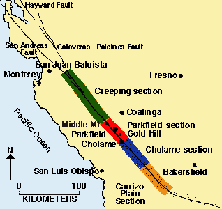Figure 1. The San Andreas Fault in central California

Figure 2 shows a comparison between observed and synthetic seismograms. The lower figure set shows a seismogram comparison between the synthetically computed and observed seismogram, computed using PREMAN, and the upper set is from IASPEI91 earth model. The travel time of some wave phases is expressed as vertical lines in the figure, which is calculated by TTIMES from IASPEI91 earth model. A set of picture consist of three traces, the lowest trace shows the vertical movement in z component, the middle is for radial component and uppers is for transversal component. The abscissa axes is the time after the Origin Time, the tick marks distance is in minutes, while ordinate axes is to express the amplitude comparison.

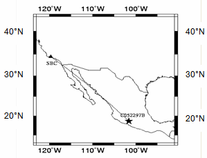Figure 2. Ray path from epicenter to SBC station

Figures 3 and 4 present seismogram comparison between data and synthetics, where lower figure set is formed from PREMAN and upper is IASPEI91 model. Figure 3 shows seismogram comparison between data and synthetics at time window of P wave. It can be seen, that P waveform from IASPEI91 arrives slightly behind the real P waveform, but the synthetic P repetitive waveform that arrives on 7 minute, has bigger amplitude than the observed repetitive P. Meanwhile the synthetic P waveform from PREMAN shows early arrival time than the observed P, while the synthetic from PREMAN in 7 minute arrives considerably early. There is no notation for this wave phase, not given by program TTIMES, but this phase is clearly not the PPP wave, because due to small epicentral distance, the arrival time of this phase arrival is not far from PnPn wave arrival time. This is also not the depth phase, because the PcP wave arrival time starts to come in 8'46". Thereby, GEMINI method that is used to calculate the synthetic seismogram gives the complete seismogram for all wave phases.

Figure 4 shows seismogram analysis at time window of S wave until the surface wave. Seismogram analysis on the synthetic seismogram from PREMAN in z component shows that this synthetic arrives earlier than the observed S, while the synthetic S from IASPEI91 arrives much earlier. For a while on t component the synthetic S from PREMAN shows a relatively good arrival time, whereas synthetic SH phase from IASPEI91 arrives earlier than real SH. Further analysis is conducted on Love surface wave. It can be seen, that waveform from synthetic Love from PREMAN is good compared to the observed Love waveform, but the synthetic Love arrives earlier than the observed Love, while waveform from IASPEI91 gives a bigger amplitude and longer oscillation. Based on the waveform comparison at Rayleigh wave, it shows that the synthetic from both standard earth models deviates far away from the observed Rayleigh wave. The arrival time difference between the main waveform and the observed data is 27 second. This is big enough, because epicentral distance is only 22.4⁰ and this is also bigger than the other arrival time difference.

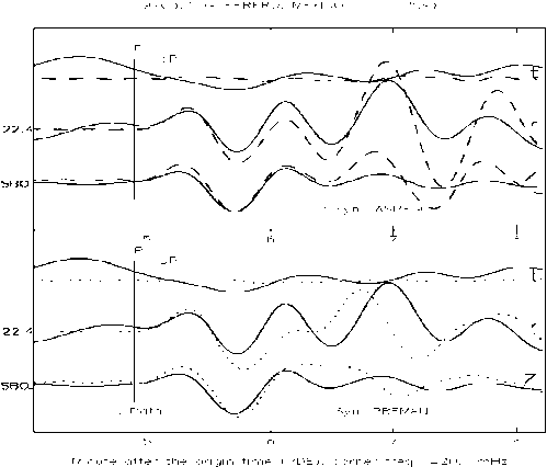Figure 3. Seismogram comparison in observation station SBC between the data and synthetics one from PREMAN and IASPEI91. Time window for P wave

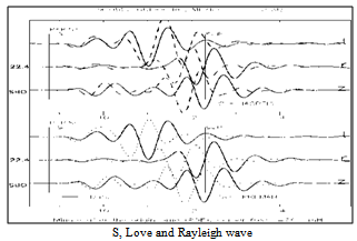Figure 4. Seismogram comparison in observation station SBC between the data and synthetics one from PREMAN and IASPEI91. Time window for S, L & R Wave

After observing some deviations that is met by seismogram comparison above, this research is aiming to achieve the fitting of surface wave, because this wave propagates on shallower earth layers, that is covering the arrival time and oscillation amount in Love wave and arrival time of Rayleigh wave. Surface wave propagates as long as Earth surface till a depth which is equivalent to the surface wavelength[21]. Therefore speed structure in upper mantle will be altered, in such a way until the fitting between seismogram observation and synthetic is achieved. Besides, it will be seen whether corrective result at structure of S wave velocity at deeper layers will give also good fitting to the S wave. It will be further investigated whether structure of S speed give the contribution for P wave, which will be shown at following analysis.

The IASPEI91 earth model is formed only from travel time data so that elastic parameters yielded are only speed of P and S wave. It is a surprise that IASPEI91 earth model can give better fitting than PREMAN model on Love wave, whether this effect only comes due to the difference in earth crust thickness. Beside that IASPEI91 earth model is in the form of an isotropic earth, though seismogram comparison the surface wave explains itself, that an anisotropic earth model shall be used to execute the inversion of both kinds of surface wave simultaneously. Therefore further seismogram comparison are relied on seismogram synthetic yielded from earth model PREMAN and corrected earth model.

Wave velocity correction is done at upper mantle layers, where changes cover the utilization of positive gradient for the and zero order coefficients of polynomial speed function for the and in upper mantle layer, while speed gradient for the is left like the initial PREMAN model. Result from this correction can be seen at Fig.5 for the time segment of P wave, where synthetic P from the corrected earth model has equal arrival time as real P, as well as waveform of repetitive P which can be better simulated. Nevertheless, it is the observed wave phase which arrives at the minute 7'48" that is still difficult to simulate, because correction is only done at S speed only. This is the topic for other seismologist to explain this P repetitive wave.

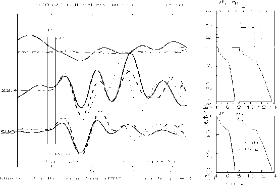Figure 5. Seismogram fitting in observation station SBC in time windows for P wave

Figure 6 shows seismogram comparison at time window of S wave until Rayleigh wave. It is interesting that fitting at all of the wave phases is achieved, starting from S wave, Love wave till Rayleigh wave and at three Cartesian components simultaneously. Fitting for the Rayleigh wave at z and r components is done only by altering zero order coefficients of speed polynomial function, the in upper mantle, while for the Love wave the corrections cover the gradient and zero order coefficients. To correct the S wave is by changing the speed on layers till 771 km depth, where the correction order is much smaller, below 0.5%. But corrections for the and requires different values, because the delay of synthetic SV and SH is different. This indicates that the anisotropy is met until the layers below the upper mantle.

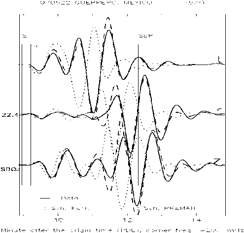Figure 6. Seismogram fitting in observation station SBC in time windows for S, L and R waves

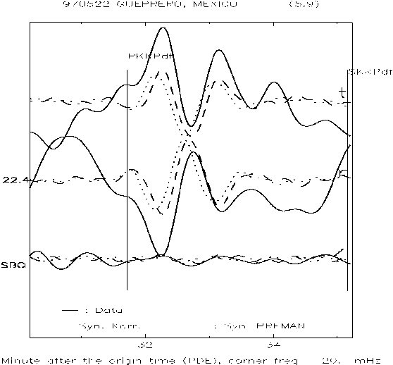
Figure 7 and 8 show seismogram analysis on core reflected ScS and ScS2 wave. It can be seen that synthetic ScS waveform from corrected earth model fits well with the observed ScS waveform. To achieve this fitting a speed correction on and till CMB is conducted. Waveform analysis on the ScS at epicentral distance as small as 23°, gives new means to investigate the structure of S velocity from upper mantle to CMB. The ScS and ScS2 waveform analysis gives better method compared to differential travel time method of SKKS and S-SKKS wave, in which this method investigate the velocity structure near CMB, that needs to be observed on seismic stations with big epicentral distance (above 83°)[10,11].

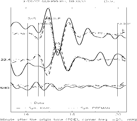Figure 7. Seismogram fitting in observation station SBC in time windows for ScS wave

Figure 8. Seismogram fitting in observation station SBC in time windows for ScS2 wave

From figure 3 above we have seen how far the deviation resulted by seismogram comparison between observed and synthetics from standard earth models is, if the analysis is carried out in time domain and three Cartesian components simultaneously. Although corner frequency of a low pass filter is set at 20 mHz, in the reality the waveform comparison give indication that the waveform is very sensitive to earth model.

Table 1. The velocity structure of S wave between the PREMAN earth-model and the corrected model of the earth for the C052297B earthquake in the SBC station; the zero-order coefficient and, on the upper mantle (6151 – 6346.6 km), the velocity gradient  is also shown

To obtain the S wave velocity structure, waveform analysis in time domain gives better result compared by noting the arrival time of S wave, which is not so easy due to lower frequency and especially in noisy time series. The dispersion analysis method measures the indirect data from seismogram that is dispersion curves for the phase/group velocity to frequency. These kinds of data were intensively used in seismology to determine the earth model.

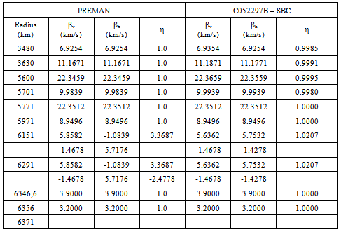
Table 1 presents the S-wave velocity on various earth mantle layers, in which the PREMAN earth-model was compared with the corrected model of the earth between the C052297B earthquake hypocenter and the SBC observation station. We can see that the vertical anisotropic ( value) occurs on all of the mantle layers, not only on the upper mantle layer as stated in the PREMAN earth-model. We notice further by comparing the second and third columns of the Table with each of the fifth and the sixth column that generally has positive anomaly on the velocity structure of S-wave occurred on all layers of mantle.

We found that the velocity structure of S wave should be corrected with the positive values down to the lowest layer of mantle i.e. CMB (3480 km). These corrections indicate that the features of vertical anisotropic are possessed by each of earth mantle layers. The validity of all magnitude of the correction should be ensured by analysing the core reflected waves, in which this wave travel passes all mantle-layers many times. This research analyses the core reflected waves at a small epicentral-distance station, in which enables us to investigate the base mantle structures near the earth core. It is different with the yielded travel-time based research of seismogram, in which they need observational data on stations with a great epicentral distance.

4. Conclusions

Seismogram data from C052297B earthquake, Guerrero, Mexico has been analysed at SBC station. The seismogram comparison is executed in time domain and three components simultaneously. Both seismograms were a low-pass filter with corner frequency at 20 mHz. In this research, two standard earth models are tested through the seismogram comparison using GEMINI program that is a program to calculate complete synthetic seismogram. There is unsystematic deviation between observed and the synthetics waveform from both models of standard global earth at various phases of surface wave, body waves and core reflected waves.

To accomplish the deviation, S speed model in upper mantle is altered to positive gradient for S speed and changes in values of zero order coefficients for the and in the upper mantle and change in earth crust thickness. This brings good fitting to surface wave of Love and Rayleigh simultaneously. To accomplish the deviation of body wave, the speed model at layers until the depth of 771 km is altered in such a way that the fitting of S wave is achieved. To obtain the fitting of deeper waves such as ScS and ScS2 the speed change is carried out until layers in base mantle. This method gives new way to investigate the S speed structure near CMB using station with small epicentral distance. In several stations, the change of S speed structure gives also the contribution to the solution of deviation at P wave.