-
Paper Information
- Next Paper
- Previous Paper
- Paper Submission
-
Journal Information
- About This Journal
- Editorial Board
- Current Issue
- Archive
- Author Guidelines
- Contact Us
Geosciences
p-ISSN: 2163-1697 e-ISSN: 2163-1719
2012; 2(5): 112-116
doi: 10.5923/j.geo.20120205.02
Prediction of Aquifer Drawdown Using MODFLOW Mathematical Model (Case Study: Sarze Rezvan Plain, Iran)
 Abstract
 Reference
 Full-Text PDF
 Full-Text HTML
A. Purjenaie , M. Moradi , A. Noruzi , A. Majidi
Watershed management, Natural Resources Faculty, Hormozgan University, Iran
Correspondence to: A. Majidi , Watershed management, Natural Resources Faculty, Hormozgan University, Iran.
| Email: |  |
Copyright © 2012 Scientific & Academic Publishing. All Rights Reserved.
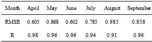
Prediction of aquifer drawdown is necessary for the correct management of an aquifer. The use of mathematical models is one important tool to predict the status of an aquifer drawdown. In this study, we have used the MODFLOW model to simulate the SarzeRezvan Aquifer. After having proven an excellent match between the generated model and the aquifer’s natural condition, we used this model to predict the aquifer drawdown. To simulate the change in water head under unsteady state, we used water head data from 2001-2010. The PEST computational code was used for calibration. Water head data from April to September 2011 has been used for verification. The Root Mean Square Error (RMSE) between observed and calculated (by the model) water head is 0.854, which indicates excellent agreement with the aquifer’s natural condition. Therefore, this model was used to predict the aquifer drawdown. The results of the model prediction have shown that if pumping is going to be constant for 8 years, the drawdown will be approximately 10.56 m, after 8 years.
Keywords: rediction, Aquifer, Drawdown, MODFLOW, SarzeRezvan, Iran
Article Outline
1. Introduction
- Today, depletion of water from aquifers that are the second largest source of freshwater in the world, has created a serious challenge for most countries[5]. On the other hand, technology development has caused rapid increase in water use, with a decline in the water table level. This requires serious, scientific management of groundwater resources[8]. Management of groundwater resources requires accurate understanding of aquifer performance under current conditions, and predicting the impacts of recharge and discharge. In order to predict the effects of recharge and discharge on the water table, the aquifer can be simulated[2]. Due to thehighability of ground water simulation models to be adapted to an aquifersystem and the ability of these models to predict, they provide favorable conditions for groundwater management[7]. One of the mathematical models that simulate aquifer behavior is the MODFLOW model. MODFLOW is athree-dimensional model that simulates flow in non - homogeneous,non – isotropicsaturated and unsteady porous environments[9]. Several studies have been performed worldwide that used the MODFLOW model for various fields of aquifer management.Rayne et al have simulated urban underground waterof Estrogen Bay(Wisconsin, USA) and determined the recharge place of fresh water wells in that area[14].Ramireddygari et al have examined the structural effects of basin and irrigation on groundwater levels to study the interaction between rivers, aquifers. They in order to combined surfacewater model with the MODFLOW model[13]. Thorley and Callander have simulated groundwater using the MODFLOW model in Christchurch, New Zealand. They used monthly data from 157 drinking water wells. The researchers used the PEST model to estimate hydrodynamic coefficients and aquifer recharge values during different periods and simulated the direction ofgroundwaterflow[17]. Chenini and Ben Mamou used GIS and numerical modeling to identify suitable sites for artificial recharge and development of underground water resources in Central Tanzania. They used GIS to produce thematic layers and the MODFLOW-2001 code to estimate the effects of recharge on hydrogeological system piezometricbehaviors[3]. Paul combined MODFLOW and WETPASS models to study land use effect on discharge and recharge of groundwater in eastern China. The research results showed that, in general, developments of urban and agricultural lands are the main causes of recharge reduction in their study area[12]. In this study, The SarzeRezvan Plain is one of the most important plains of Hormozgan Province (Iran) for agricultureandfresh water supply. Excessive pumping of water from the aquifer during the past two decades has caused disastrous consequences for agriculture[18]. The aquifer unit hydrograph shows a drawdown of 6 meters from 1999-2008 (Fig.2). The aim of this study is to predict the SarzeRezvan Aquifer drawdown using the MODFLOW mathematical model after to investigate adaptation of the model to the aquifer’s natural conditions.
2. Data and Methodology
2.1. Study Area
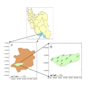
- SarzehRezvan Plain has an area of about 7600 hectares and is located approximately 52 kilometers northwestof Bandar Abbas City in the Hormozgan province, Iran. This plain extends between of 56° 03' to 56° 11' longitude and 27° 33' to 27° 36' latitude. The minimum elevation is 330 meters and its maximum elevation is 400 meters. There are 181 wells located in the plain. The number of observation wells is 10. This plain has an average rainfall of 161.95 mm. Figure (1) showsSarzehRezvan Plain location.
 | Figure 1. Location of the SarzehRezvan Plain |
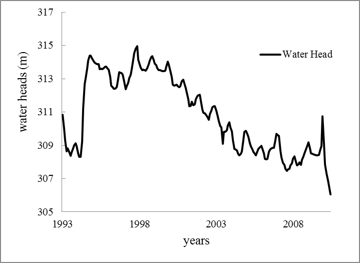 | Figure 2. The aquifer unit hydrograph of SarzeRezvan plain |
2.2. Study Method
2.2.1. AquiferModel Designand Calibration
- Necessary information to simulate the aquifer using the MODFLOW model are: the surface and bottom topography of the aquifer, precipitation and evapotranspiration values, utilizationwell characteristics and statistics, amount ofirrigationwater, type ofcropcultivation, surface water sources and relation to groundwater, preparation ofobservation and exploratorywellsections, layer textureandgeologicaldata, determination of boundary conditions, observationwell levels, and the aquifer hydraulic conductivity and storage coefficient. After collecting the above mentioned information, the finite difference grid was designed such that the number of columns and rows were 103 and 40, respectively, with grid dimensions of 150×150 m. In addition, the aquifer was determined to be unconfined and of a single-layer according to geophysical and geological information. The aquifer surfacetopographicmap (scale, 1:25000) was digited by ArcGIS9.3 software and entered into the model with ASCII format. The aquifer bottom level map was calculated from the difference between the aquifer surface level map and depth to bed rock map, then was entered into the software. The depth to bed rock map was prepared by the Geophysics Department[10]. The aquifer’s physical and hydraulic boundaries were defined according to topographic, geological and groundwater level maps and surface rivers location for determination of aquifer boundary conditions. Also for determination of aquifer boundary conditions, the cells were identified as active or inactive. Figure 3 shows the aquifer boundaries, designed grid, and type of cells. According to The aquifer unit hydrograph (Fig. 2), from the beginning of the statistical duration until approximately 2001, the aquifer’s balance was about zero. Therefore, we used 2001 as the simulation start time. Data from 2001-2010 was used for model calibration in the unsteady state. To determinate the number and length of model periods in the unsteady state, the unit hydrograph is used. According to the unit hydrograph, an increase and decrease was observed in the water level for all of the years. The increase in water head was related to the April to September of each year (spring and summer, first periods) and the decrease in water head was related to the October to March (fall and winter, second periods). Thus, each statistically years divided into 2 time periods and total statistical period was divided into 20 time periods. Well pumping in the second period was almostdouble when compared to the firstperiod due to cultivation of specific crops[4].In this model, we entered the water heads of the observation wells, hydraulic conductivity, storage coefficient, effective porosity, aquifer discharge (according to pumping statistics) and aquifer recharge. In this plain, the majority of aquifer discharge occurs from utilization wells. Aquifer recharge may be estimated by conventional methods such as water-balance, Darcian approach, lysimeter, water table fluctuation and numerical simulation method[16,15,11]. In this study, recharge values were determined by the numerical simulation method. The main model was calibrated by the PEST code in an unsteady state with data from 2001-2010 (10 years, 20 time periods). The PEST code is a software package for nonlinear parameter estimation that can run themodel numerous times until computational and observational parameters areclosedtoeach otherin order to reach the least weighted squares. The aim of the PEST code is to help with interpretation, parameter calibration and predictiveanalysis. This code is connected to MODFLOW[6].
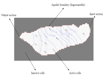 | Figure 3. Aquifer boundaries, designed grid, and cell types |
2.2.2. Model Verification
- An accurate model is a model that in addition to simulate of water head in calibration period, it can simulate water head for another stress period, with the same accuracy of calibration period[1]. After the model was calibrated from 2001-2010 (20 time periods), data from the April to September of 2011 was used to verify the made model for SarzeRezvan Aquifer. However, the needed information for the 6 months was entered into the model and it was assumed that the stress change was similar to previous years. But observation heads for these six months were not entered into the model and the model was subsequently run and the water head was calculated. Then, the model’s calculated heads were compared with the observed heads.
2.2.3. Aquifer State Prediction
- A model that has passed the calibration and verification stages would be suitable for future prediction of the aquifer state. We can present the most accurate prediction for the aquifer, with predicting all the parameters for an aquifer system. Hence, we can enter into the model the different parameters based on previous years as a trend to predict the aquifer’s future state or we can consider usual and unusual conditions for the model and then study the model’s responsetovarious scenarios.
3. Results and Discussion
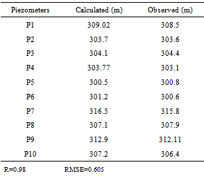
- The SarzeRezvan Aquifer model was calibrated by the PEST code in an unsteady state over a ten-year period (2001-2010). Calibration results were obtained from comparison of the calculated and observed heads in all piezometers. Figures (4, 5) show calibration results and calculated and observed hydrographs in the calibrated ten-year period in piezometer of 4 as example respectively. In these hydrographs, the thick lines represent calculated hydrographs, whereas the thin lines show observed hydrographs. The horizontal axis represents the time (days) and vertical axis is the water head (meters). April 2001 was considered the simulation start time. Time axis divisions are 360 day. As shown below, the observed and simulated (calculated) water heads have an excellent agreement. In addition, the right figures show the calibration results and correlation between observed and calculated heads with their variances. In these figures, the variance between observed and calculated heads is low, therefore, the model has an acceptable accuracy.
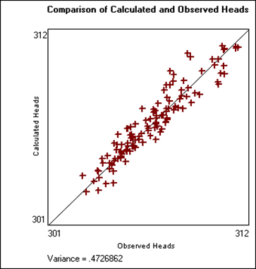 | Figure 4. Comparison of the calculated and observed heads in Piezometerof 4 |
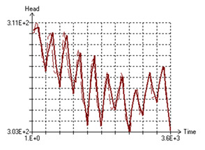 | Figure 5. Comparison of the calculated and observed hydrographs inPiezometerof 4 |
|
|
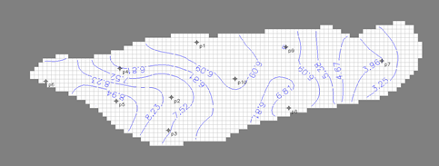
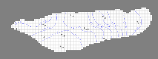 | Figure 6. Prediction of aquifer drawdown with constant pumping after 8 years |
 | Figure 7. Prediction of aquifer drawdown with 20% decrease in pumping after 8 years (meter) |
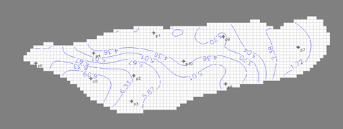 | Figure 8. Prediction of aquifer drawdown with 40% decrease in pumping after 8 years (meter) |
|
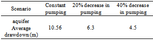
4. Conclusions
- To verify the created SarzeRezvan Aquifer model, we used the correlation coefficient (R) and RMSE between observed and calculated water heads from April to September of 2011. The RMSE between observed heads and calculated head by model was 0.854 and the correlation coefficient (R) between them was 0.94, which both show excellent agreement of made model with aquifer’s natural conditions. Therefore, the model was used to predict the aquifer drawdown. The results of the model prediction show that if the pumping is kept constant during 8 years, the drawdown will be approximately 10.56 m, after 8 years. Also, the aquifer drawdown will decrease to 6.3 m if the aquifer pumping value decreases 20% during 8 years and the aquifer drawdown will decrease to 4.5 m if the aquifer pumping value decreases 40% during 8 years (than 2011). The most aquifer drawdown was noted in the western range of the plain (near Rezvan village). Because In this region, there is a high concentration and high pumping of utilization wells. In general, with the current pumping trend, the aquifer will not be responsive to pumping, which may cause a threat to agriculture. In the end, we suggest that in future studies, to increase of accuracy in the Prediction of Aquifer Drawdown using MODFLOW, the first, predict the aquifer recharge by advanced models and then define the scenarios for model.