1. Introduction

One of the tools of investigating the thermal framework via aeromagnetic studies is spectral analysis. In the last few decades, spectral analysis based on statistical models has been used in various geological applications like the estimation of average depth to the top of the magnetic basement and the estimation of crustal thickness. This spectral method pioneered by[25] has been used extensively in the interpretation of magnetic anomalies. It is based on the expression of the power spectrum for the total field magnetic anomaly produced by a uniformly magnetized rectangular prism[1]. [25] assumed that a number of independent ensembles of rectangular prismatic blocks are responsible for generating anomalies in a magnetic map.

[1] defined CPD as “the deepest level in the earth crust containing materials which creates discernible signatures in a magnetic anomaly map”. This definition can then be restated as saying that CPD is the depth at which the Fe-Ti Oxide minerals of the Earth lose their ferromagnetic property[13]. This Curie Isotherm has a temperature of 550℃ ± 30℃. This point is assumed to be the depth for the geothermal source (magmatic chamber) where most geothermal reservoirs tapped their heat from in a geothermal environment. CPD provide general information on both regional and local temperature distribution as well as geothermal gradients[9]. Curie Point Depth offers a window for a better view of the thermal structure of the crust via aeromagnetic data as the difference between short wavelength and long wavelength anomalies can be an indication of CPD.

In Nigeria, extensive geophysical investigations have been largely confined to sedimentary formations with proven natural resource potentials. The Niger Delta area of Southern Nigeria has witnessed extensive gravity, magnetic and seismic surveys in connection with oil and gas prospecting by oil companies operating in Nigeria. The Chad Basin has also attracted some attention of recent because of the suspected propensity of the area in terms of oil and gas.

[13] estimated the depth to the Curie Point Isotherm of the Upper Benue Trough by subjecting the residual data obtained from that area to Upward continuation in order to remove the component of the field due to shallow sources and also carried out a Two-dimensional spectral analysis and Hilbert transformation of aeromagnetic data over the Upper Benue trough in order to estimate the depths to magnetic sources and also delineate the major structural patterns in the study area. Their result show that the Curie point isotherm of the region varies between 23.80km and 28.70km. The deeper magnetic sources depth of up to 3328 m was obtained, representing the sedimentary cover in the study area. The highestdepth to the shallower magnetic source model is 830mand represents intrusive/extrusive bodies within the trough. [15]carried out the aeromagnetic investigation of the geothermal source potential of part of the Niger Delta. He used Spectral analysis to obtain the Curie Point isotherm of the region to vary between 5.73km and 12.97km.

This work is aimed at filling the missing gap in the crustal temperature information of the study area in addition to providing clues to likely productive zones for geothermal exploitation.

2. Geology of Study Area

The study area lies in the East Central part of Nigeria and lying between Latitude 7°N and 9.5°N and Longitude 9.5°E and 12°E. The area is represented by twenty – five (25) Topographic maps compiled by the Nigeria Geological Survey Agency (NGSA). The maps include 191 – 195; 212 – 216; 233 – 237; 253 – 257 and 273 – 277. One of the most prominent geological landmark in the area is the Benue Trough which runs through part of the area along a SW – NE trending.

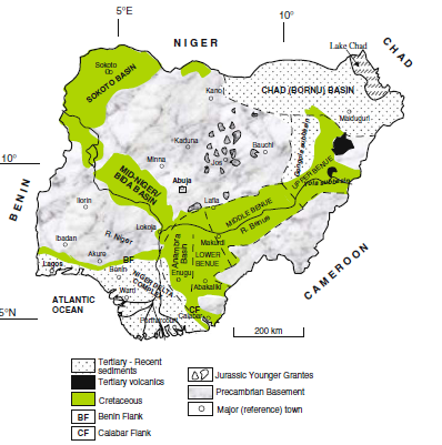Figure 1. Geological map of Nigeria showing the study area afterObaje(2009)

The study area is a square block situated at the east central part of Nigeria. It is bounded by Latitudes 7°00’N and 9°30’N and Longitudes 9°30’E and 12°00’E. The area lies around the sedimentary formation of the Middle Benue Trough and partly in the basement complex region of North Central Nigeria.

The Benue Trough originated from Early Cretaceous rifling of the central West African basement uplift. It forms a regional structure which is exposed from the northern frame of the Niger Delta and runs north-eastwards for about 1000km to underneath Lake Chad, where it terminates.

Regionally, the Benue Trough is part of an Early Cretaceous rift complex known as the West and Central African Rift System. It is a linear rift system whose development was closely associated with the separation of Africa from South America and the opening of the South Atlantic Ocean. Geological studies have shown that the trough was subjected to several depositional cycles which resulted in the deposition of sedimentary rocks of varied compositions and ages[8,19]. Three of these depositional cycles were more pronounced than the rest. The first major sedimentary cycle lasted from the Middle to the Late Albian and marked the initiation of sedimentation in the trough. This cycle began with the Middle Albian transgression which was marked by the deposition of the predominantly black shales of the Asu River Group. The regression which marked the end of this cycle lasted from the end of the Albian to about the end of the Cenomanian and was associated with the deposition of the Keana and the Bima Sandstones. The second sedimentary cycle began with a transgression at the end of the Cenomanian and ended with a regression in the Early Turanian. Associated with the transgressive and regressive phases of this cycle was the deposition of the EzeakuShales and deltaic Makurdi Sandstones respectively. The third major sedimentary cycle in the Benue Trough occurred from the Late Turanian to the Lower Santonian and most deposits associated with this cycle are believed to have been eroded as a result of a Late Cretaceous tectonic activity, while its regressive phase was accompanied by volcanic activity in the Upper Benue Trough[8,17].

The younger granite complexes in Nigeria are found mainly on the Jos Plateau, forming a distinctive group of intrusive and volcanic rocks that are bounded by ring dykes or ring faults. Other occurrences approximate a north-south belt towards the middle Benue in the south where the ages are younger, and towards Niger Republic in the north where the younger granites are older. There is enormous variety in the granite composition of these rocks. The younger granites form rugged hills of Jurassic age, and contain tinstone and columbite. Valuable deposits of these minerals have been formed from the disintegration by weathering of the granites. The concentration of these ore minerals is present in stream beds of earlier and recent geological epochs. Small quantities of wolframite also occur in certain Younger Granites, and some contain the potentially valuable radioactive mineral, pyrochlore. The Mesozoic Younger Granite ring complexes of Nigeria form part of a wider province of alkaline anorogenicmagmatism. They occur in a zone 200 km wide and 1,600 km long extending from northern Niger to south central Nigeria. Rb/Sr whole rock dating indicates that the oldest complex of AdrarBous in the north of Niger is Ordovician in age, with progressively younger ages southwards. The most southerly ring complex of Afu is Late Jurassic in age[4]. Aeromagnetic anomalies suggest that a series of buried NE–SW lineaments of incipient rifts controlled the disposition of the individual complexes.

About half of Nigeria is underlain by crystalline rocks. The rocks are exposed in three large areas, namely, the northern, western and eastern parts, and they consist of series of granites, gneisses, migmatites and narrow belts of low-grade schists, quartzites and amphibolites. Collectively, the rocks are known as the basement complex and they are Precambrian in age. The rocks were formed as a result of metamorphosis and igneous activities on a regional scale. Basement complex rocks are subdivided into migmatite-gneiss complexes; the older metasediments; the younger metasediments; the older granites; and the younger granite alkaline ring complexes and volcanic rocks. The migmatite gneiss complex is the commonest rock type in the Nigerian Basement complex. It comprises two main types of gneisses: the biotite gneiss and the banded gneiss. Very widespread, the biotitic gneisses are normally fine-grained with strong foliation caused by the parallel arrangement of alternating dark and light minerals.

3. Data Acquisition

The data used for this research were published in the form of ½^oby½^o aeromagnetic maps contoured at 10nT intervals. Twenty five (25) such maps obtained from the Nigerian Geological Survey Agency (NGSA). The maps are 191 – 195; 212 – 216; 233 – 237; 253 – 257 and 273 – 277. The composite map for the East Central Nigeria comprises of twenty-five (25) sheets with regularly spaced grid points. The composite map was then subjected to polynomial fitting for Regional and Residual Separation. The map below is the residual map of the study area from Oasis Montaj software by Geosoft.

4. Methodology

The Spectral depth method is based on the principle that a magnetic field measured at the surface can be considered as the integral of magnetic signatures from all depths. The power spectrum of the surface field can be used to identify average depth of source ensembles. This same technique can be used to attempt identification of the characteristic depth of the magnetic basement, on a moving data window basis, merely by selecting the steepest and therefore the deepest straight-line segment of the power spectrum, assuming that this part of the spectrum is sourced consistently by the basement surface magnetic contrasts. A depth solution is calculated for the power spectrum derived from each grid subset and is located at the centre of the window. Overlapping the windows creates a regular comprehensive set of estimates.

The methods of Curie Point Depth determination utilize spectrum analysis techniques to separate influences of the different body parameters in the observed magnetic anomaly field. The signal from the top surface of a magnetized body dominates the signal from the bottom at all wavelength which makes the inverse problem more complicated[3]. Fundamentally, the method of[25] estimates the average depth to the top of an ensemble of magnetized rectangular prisms from the slope of the log power spectrum while the method of[1] obtains the depth to the centroid of the causative body using a single anomaly interpretation. [20] effectively combined and expanded the ideas of both methods proposing an algorithm for regional geomagnetic interpretation oriented to the purposes of geothermal exploration. They considered a two-dimensional modelling technique for determination of depth to the base for a single block with the average parameters of the ensemble. Their algorithm estimates the depth to the centroid, () from the slope of the radially averaged frequency-scaled power spectrum in the low-wave number part and depth to the top from the slope of the radially averaged power spectrum (RAPS) where is radial frequency. The bottom depth is then obtained from

.

The method of[26] is quite similar to the method so described above. They used both the high wavenumber and low wavenumber parts of RAPS. They estimated the top bound of magnetic source by fitting a straight line through the high-wavenumber part of RAPS and respectively the centroid () by fitting a straight line through the low-wavenumber part of frequency-scaled RAPS where is the power density spectra and is the wavenumber. The basal depth was also calculated from.

The study area was divided into twenty–five overlapped blocks for the purpose of spectral analysis as shown in Figure below. Each block covers a square area of 55 Km by 55 Km.

Power spectral analysis was conducted on the residual values of each of the blocks by plotting the logarithm of spectral energies against the frequency. This reveals graphs whose linear segments have gradients that are a function of the depths to the ensembles causing the anomaly. The group of such blocks is treated by statistical theory and reduced to power spectrum. The result of the analysis is plotted on a logarithmic scale against the frequency. On such a plot, if a group of sources has a similar depth, they will fall into a line of constant slope. Thus if there are groups of sources with individual groups at widely different depths, such as shallow volcanic over a deep basement, the plot will be separable into parts with different slopes and the magnitude of the slope is a measure of depth.

This process was carried out for the twenty five blocks to obtain the depth to shallow and deep causatives. The Curie point depth for each block was then obtained using the formula .

The Figure below is the map of the Curie point isotherm of the study area.

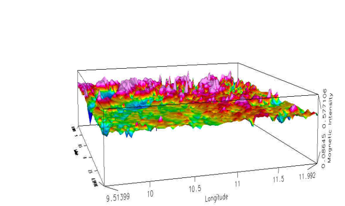Figure 2. 3D view of the Residual Magnetic field of the study area

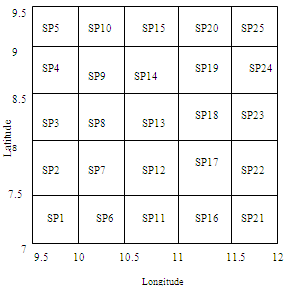Figure 3. The layout of the field of study into units of blocks for spectral analysis

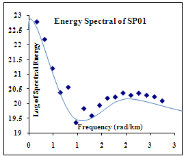Figure 4. Result of spectral analysis for SP01

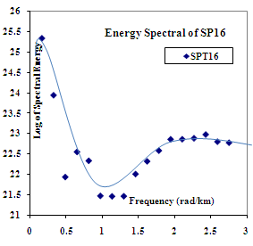Figure 5. Result of spectral analysis for SP16

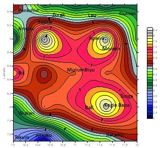Figure 6. Curie Point Isotherm for the study area

5. Results and Discussion

From the graphs of the Logarithm of spectral energies versus frequencies plotted for each block, there were spectral peaks which were easily noticeable and the significance of this is the indication of the fact that Curie point depths are detectable as it defines the source bottoms. Figure 6 shows the result of the investigation of the Curie Point Isotherm of the study area and it reveals the Curie isotherm depth varies between 2 and 8.4 km. A closer look at the figure also reveals that the shallowest region lies at the south western region of the study area. Generally, the Curie point depths are shallower than 15km and this, according to[26] reveals that the entire area is volcanic and geothermal field since Curie point depth is greatly dependent on geologic conditions. Particularly the south western portion of the study area where the curie point depth is shallowest. The central portion of the study area shows relatively high values of CPD and the contour in Figure 6 shows a NW – SE trending. The entire area is recommended for more geothermal reconnaissance investigation.

6. Conclusions

The difference in frequency characteristics between the magnetic effects from the top and bottom of the magnetised layer in the crust can be used to separate magnetic effects at the two depths and to determine the Curie depth. The isotherm has, therefore, been determined in the eastern sector of central Nigeria and it is found to vary between 2 and 8.4km. In the southwest of the study area, bounding Atsuku, Takum and Wukari, the curie-depth was found to be lowest at about 2.4km, while it was found to peak at depths of about 8.4 km in the central parts around Apawa, Monkin and Kogin Baba.