1. Introduction

About 50 million years ago (Early Eocene), south eastern Eurasian plate faulted to the southeast and composed the western region of Indonesia. Piercing plane started on the Late Mesozoic in the western of Sumatra, it is weakening at Paleocene and stopped at Eocene.

As a tectonic region, Sumatra Island consists of two main parts, the west is dominated by the oceanic plate and the east is dominated by continental plate. Based on the measurement of gravity, magnetism and seismic ocean plate thickness of about 20 kilo meter, and the thickness of continental plates about 40 kilo meter[1]. Tectonic history of the Sumatra island is closely linked to the start of the collision among the Australian and Eurasian plates, about 45.6 million years ago, which resulted in a series of systematic changes of the relative movement of plates followed by changes in the relative velocity among the plates followed by extrusion events.Australian plate that moves to northwest in average rate of 5.5 to 7 cm/year and Eurasian plate that moves to the southwest in average rate of 2.6 to 4.1 cm/year[2].

Based on morphological characteristics, Sumatra is divided into several zones. There are Central - South Sumatra and North Sumatra - Nicobar. The Central and South Sumatra have the depth of the subducted zone that gradually reduced from 6000 to 5000 m. Sediments located at the bottom part of trench have a thickness of about 2 km in the north and 1 km in the south. The subduction plane movement bent to the north with a decreasing from 7.0 to 5.7 cm/year. Components of the lateral shift that work in this plate assumed to have very important role in shaping the strike slip fault system in Sumatra.

In the zone of North Sumatra, Nicobar, in the west of the Simalur Island, the trench axis sharpened to the west, and in the northwest of Simalur tend to bend to the north - northwest. Trench has a depth ranging from 3500 to 5000 m. The meeting along this zone is bent and the speed of piercing toward the north decreased from 5.6 - 4.1 cm/year.

In last two decades, the global seismic tomography has routinely processed the travel-time data, for example International Seismological Center (ISC). This routine became especially very successful in three dimensional subduction of the cold oceanic crust beneath the continental earth crust mapping, along the front region of the active trench.

According to Replumaz et al.[3], in front region of the subduction zone, the continent edge experiences compression which is caused by collision of the oceanic crust, the P velocity structure in the upper mantle layer has positive anomaly. Such velocity structure is obtained by inversion of the direct P travel time data using ≈ 8 × 10⁶, the reflected P wave phase ≈ 0.6 × 10⁶, and the biased PKP in earth's core ≈ 1 × 10⁶. This numerous amount of data are gathered from 300,000 earthquakes, recorded from time range 1/1/1964 to 31/12/2000[4-6.], also a small number of absolute time arrival difference data of PP-P, PKP-P_diff, which is measured accurately using the cross correlation waveform of the digital data broad-band[7]. The travel time and dispersion data are mostly used to interpret the earth model globally[8-10] or regionally[6,11].

The epicentral distance from earthquakes hypocenter in Sumatra-Java to UGM observatory station is small. Seismogram analysis of S wave to derive the S wave velocity structure in such small distance is not easy because of the waves crumple. So only the first break arrival time can be measured clearly. It is difficult to measure the arrival time of the S wave with appropriate accuracy. Direct measurement of the S travel time is not easy, because of arrival time differences of the P, S and the surface waves is very short, whereas the amplitude of the S wave is smaller than the surface wave. The ISC routine rarely includes the S wave travel time in such small epicentral station. So that the amount data of S wave travel time is only 2% of P wave travel time[8]. The data set analysed in this research is the seismogram waveforms, from surface wave to S, ScS and ScS₂ waves, instead of the travel time data. Although the data set used by other seismologists includes millions of travel times in number, it contains just a little of information in the seismogram time-series. In contrast, the waveforms of the S, ScS and ScS₂ waves, the Love and Rayleigh surface waves in the three Cartesian components, carry all information of the seismogram.

Up to-date, seismological researches[12,13-15] which interpreted P and S wave velocity structure in subduction zone still use travel time data, whereas the data were measured from seismogram which are triggered by local earthquakes or teleseismical data. Replumaz et al.[3] has interpreted the model of the P velocity anomaly which is taken from the travel time data of the P wave only. To obtain this anomaly, the initial earth model used is the isotropic earth model, because the anisotropic model in the earth is difficult to be researched using arrival time data. In an isotropic homogeneous medium the relation between these two velocities models is. Therefore it can be assumed, that the β anomaly takes also the form of α anomaly. The upper mantle layers in the earth layering system is laid from depth 30 km down to 240 km, is used to represent the values of the α anomaly in the upper mantle. According to Replumaz et al.[3] the Sumatra and Java Islands has positive velocity anomaly.

This research investigated the β velocity anomaly in the same region (small piece of Replumaz et al.[3] region, Sumatra-Java) using seismogram analysis in time domain and three Cartesian components simultaneously. The objective of this research is to investigate whether the front region of subduction zone has positive β velocity anomaly, as supposed from P wave anomaly[14].

2. Method and Data

This research completed the S velocity structure in the Sumatra-Java Islands that is located in front region of the subduction zone. The earthquakes occurred along the Sumatra Island, from Nicobar, Northern Sumatra, until the Sunda Strait, the seismogram triggered by these earthquakes will be analysed, which were recorded in the UGM station. Table 1 presents the positions of earthquakes epicenter and the analysed seismogram were recorded in UGM observatory station. Figure 1 presents the vertical projection of seismic wave paths from earthquakes epicenter to UGM observatory stations.

Table 1. List of earthquakes which seismogram is analysed in UGM No Earthquake Code Latitude Longitude Location 1 B031501B 8.66 94.01 Nicobar Islands 2 C110202J 2.95 96.39 Northern Sumatra 3 C011601D -4.02 101.78 Southern Sumatra 4 B122901B -6.01 102.85 Southwest Sumatra 5 C102500D -6.31 105.21 Sunda Straight 6 C062702C -6.96 104.18 Sunda Straight

To identify the wave phase in the seismogram, the TTIMES program was used, which is downloaded from www.orfeus-eu.org. Whereas the GEMINI program (Green function of the Earth by MINor Integration,[16,17]) is used to calculate the synthetic seismogram in the time domain and three Cartesian components simultaneously. This method calculates the minors of the Green functions for a vertical anisotropic earth model with a certain depth of the earthquake source and location of the station. The Minors of Green functions are expanded into spherical harmonic functions by fulfilling the boundary conditions in the deepest (reflected) point of wave propagation, the source depth point and the earth surface. The independent variable is the complex frequency (ω+ισ), to avoid time aliasing. These Minors of Green function are then multiplied with the spherical harmonic and the moment tensor of the earthquake which also has been expanded in spherical harmonic functions. The degrees for spherical harmonic expansion are determined from the epicentral distance and azimuth of the recording station. The program ends by summing them up to produce the synthetic seismogram which is still in complex frequency domain. This seismogram is then back Fourier transformed into time domain. Inverted Response file of the canal in the observatory station is imposed to the correspondence measured seismogram, so that the seismogram comparison is conducted in the same units. The Butterworth low pass filter is subjected to both seismograms, the measured and synthetic seismogram to simplify the waveform analysis. The corner frequency of the low pass filter was set at 20 mHz.

When the GEMINI program is run, an earth model and a certain depth of earthquake must be given as input, which is initially the anisotropic PREM (hereafter PREMAN[8]). As an input earth model, the data must contain elastic parameters completely, which covers the compression and shear wave velocities, density and inelastic parameters μ and κ of rock compiler's of the earth structure.

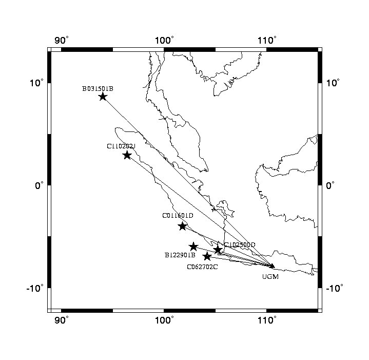Figure 1. Wave paths vertical projection from earthquakes epicenter to UGM station

The seismogram comparison shows big discrepancies between the measured Love and Rayleigh wave and the correspondence synthetic surface waves. The following figures present the seismogram comparison and fitting for Love, Rayleigh waves, and S wave to obtain the β velocity structure in shallow earth layers until 730 km depth. Each figure contains 3 trace, each presents the components of the ground movement, marked with z to vertical, r to radial and t to transversal, respectively. In each component presents 3 curves, where the solid curve is the measured data, the dotted curve presents the seismogram constructed from PREMAN earth model, and the dot-dashed curve is the synthetic seismogram constructed from the corrected earth model, where the corrected S velocity structure is displayed in the right small box as the dot-dashed curve. Generally, to get the seismogram fitting, the velocity gradient β_h in the earth upper mantle is changed into positive against the depth[16], than the negative one as stated in PREMAN earth model, while the β_v gradient is not changed. The changes are only carried out to the zero order coefficients of polynomial which depicted the S velocity function in each earth layer, by iterative method.

3. Seismogram Analysis and Discussion

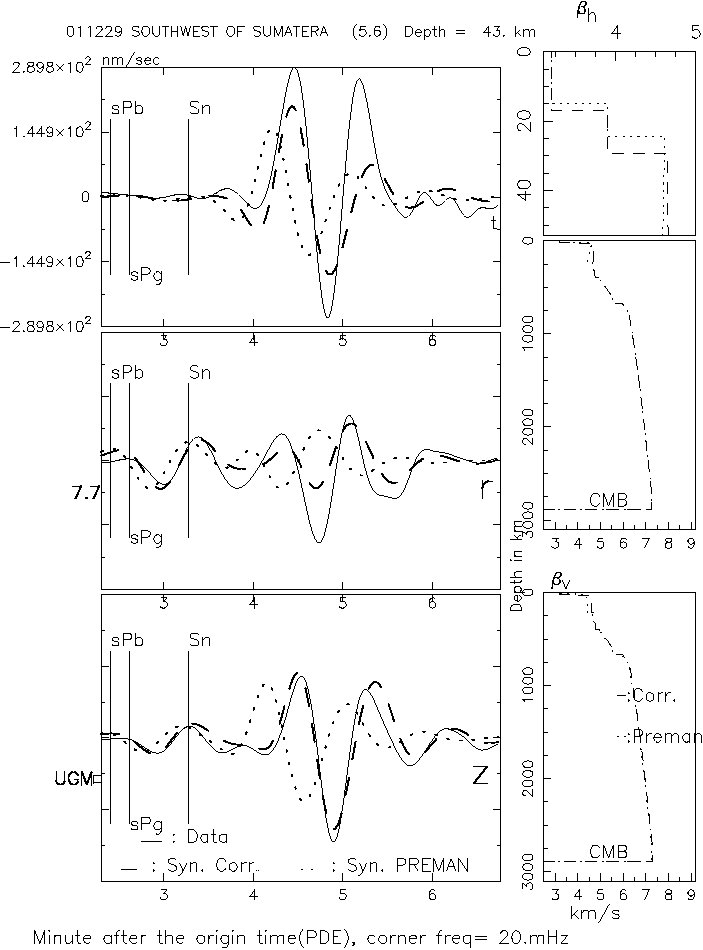
Seismogram analysis and fitting

First, the seismogram analysis and fitting of B031501B earthquake which occurred in Nicobar Islands are shown, where the data was recorded at UGM station, as illustrated in fig. 2. Fig. 2a gives illustration, that PREMAN earth model provides synthetic Love waveform, which is shorter and decayed faster than the measured Love wave. The using of positive β_h gradient in the upper mantle and thickening of the earth crust into 40 km provide excellent fitting on observed Love waveform. Further corrections on zero order coefficients of β_h until 630 km depth is carried out, to obtain the SH wave. Here we can see that earth crust thickening and S velocity structure in the upper mantle give excellent fitting to the surface wave. Rayleigh waveform is not sensitive to earth crust thickening. Fig. 2b shows, that the S velocity changing influences the synthetic P waveform which resembles the pattern of the measured P waves, although the arrival time is still later.

Further is the seismogram analysis of C110202J earthquake, Northern Sumatra, where this earthquake hypocenter located in southern part of the Nicobar earthquake hypocenter, where the recording was conducted by the UGM station. Figure 3 shows wave fitting for various body waves and surface wave. Figure 3a shows the seismogram fitting to the Love and Rayleigh surface waves, also the S body wave. We can see that the Rayleigh wave fitting can be reached only in t and r components, whereas in z component the synthetic Rayleigh wave from the corrected earth model still gives earlier arrival time than the measured Rayleigh wave. This shows that anisotropy is more complex than supposed in vertical anisotropic earth model. This result of upper mantle S wave velocity in the upper mantle is contrary to the research result of Barklage et al.[19]. Generally, we can see that the anomaly in upper mantle for these two S waves velocity is being negative for the wave path from North Sumatra to UGM. The following three figures show seismogram fitting to P and core reflected ScS and ScS₂ waves. Core reflected waves propagate in all of the earth mantle layers and earth's crust layer from the earth surface to CMB (Core Mantle Boundary) two and four times, respectively. These two core reflected phases show that the small positive velocity anomaly also occurred in earth layers below upper mantle down to CMB.

Figure 4 presents the seismogram fitting of C011601D earthquake which occurred in South Sumatra and recorded in UGM station. The figure gives the illustration concerning the fitting for S wave until Love wave, which arrival time and waveform are excellently achieved. This fitting is obtained by thickening the earth's crust 5 km than the PREMAN crust model (25 km). The Love wave is very sensitive to the Moho depth, whereas the Rayleigh wave is not sensitive to the earth's crust thickness changing. The second and third figures show fitting for the ScS and ScS₂ wave, where to fit the small positive correction in the earth mantle layers until CMB is required.

Figure 5 shows seismogram fitting in various wave phases, beginning from the P, S wave, and to the Love and Rayleigh surface wave, where the seismogram is triggered by B122901B earthquake which occurred in South Sumatra. The strong negative anomaly is occurred in the upper mantle, because the epicentral distance is close, so that this strong correction must be carried out in the upper mantle layers, to obtain the fitting on the surface wave. Small negative correction is also occurred in mantle layers below the upper mantle to achieve the fitting for S wave. Correction in β also provides the contribution to the time arrival improvement of the P waveform.

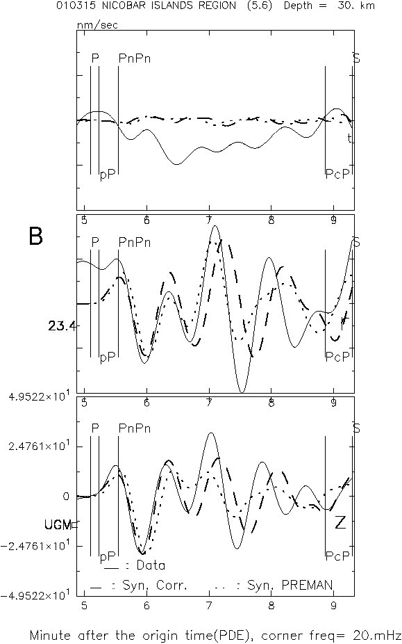Figure 2. Seismogram comparison of B031501B earthquake, Nicobar Islands at UGM station, a). S, L and R; b). P wave

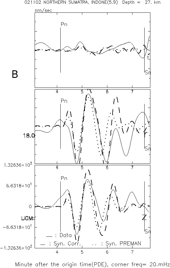Figure 3. Seismogram comparison of C110202J earthquake, Northern Sumatra at UGM station, a). S, L and R; b). P; c). ScS and d). ScS2 waves

Figure 4. Seismogram comparison of C011601D earthquake, Southern Sumatra at UGM station, a). S, L and R; b). ScS and c). ScS2 waves

Figure 5. Seismogram comparison of B122901B earthquake, Southern Sumatra at UGM station, S, L and R waves

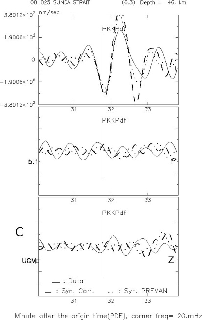Figure 6. Seismogram comparison of C102500D earthquake, Sunda strait at UGM station, a). S, L and R; b). ScS; c).ScS2 waves

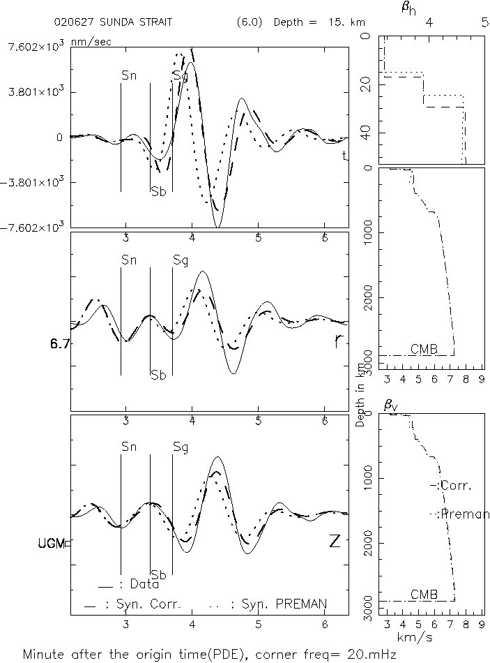Figure 7. Seismogram fitting of C062702C earthquake, Sunda strait at UGM station, S, Love and Rayleigh waves

The Hypocenter of C102500D earthquake took place in Sunda Strait, but the position is eastern from the previously analysed B122901B earthquake. Figure 6a show that negative correction in the upper mantle is required for β_h and earth crust thickness, to fit the Love waveform, but small negative corrections are also imposed to the mantle layers beneath the upper mantle, to fit the S and its repetitive wave because the arrival time is earlier than the observed Love wave, which have big amplitude in r component. This is not the Rayleigh wave, because its arrival time is later than Love wave. Fitting is achieved until the last oscillation of the Rayleigh wave. Figures 6b and 6c show that the constructed ScS and ScS₂ wave from PREMAN model arrives later than the correspondence measured wave phases. The propagation of ScS and multiple wave traverses all part of the earth mantle from the earth crust down to the CMB (Core Mantle Boundary), so that the small positive correction of β_v must be also imposed in the mantle base layers.

Figure 7 presents the seismogram comparison of C062702C earthquake between the synthetic seismogram constructed from PREMAN and corrected earth model, which is then compared to the observed seismogram. Synthetic seismogram form PREMAN provides the arrival time of S wave which is earlier than the observed S wave. Due to small epicentral distance, S wave is in front disturbance of the Love wave, where the PREMAN provide earlier and weaker Love waveform. So that strong negative corrections are carried out for the advance of S arrival time, but this effort does not brings the Love waveform amplitude which resembles the observed waveform amplitude. By doing earth crust thickening, the amplitude height is achieved. This factor is not used by seismogram analysis, whether by the travel time nor the dispersion methods.

4. Discussion

In an isotropic earth model the value of elastic parameter λ is equivalent with μ, so that it can be supposed that the, so it can be supposed that the S anomaly takes the same form as the P anomaly. Replumaz et al.[3] interpreted that the front region of subduction has positive anomaly in P wave velocity structure. This research shows that the anomaly of S wave is contrary to the result of Replumaz et al.[3]. Therefore the assumed relation between P and S wave velocities were not correct.

Castle et al.[20] interpreted that the slow wave velocities show the hot thermal sign of slabs in the upper mantle. Slow wave velocities in the mantle layers are well correlated with hotspot locations. In their 30 degree model, slow regions correlate to the surface location of hotspots, supporting their previous observations. If no correlation existed between hotspot locations at the surface and slow anomalies in the lowermost mantle, it would strongly argue that hotspots do not originate within the basal layer. The result of this research can be used to interpret the temperature of the region in front of the subduction zone that has higher temperature in the upper mantle, as consequence of compressed region due to collision between the oceanic crust and continental crust.

Yoshizawa et al.[21] used 211 seismic events from 2005 to 2007 at depths shallower than 100 km with moment magnitude (Mw) between 6.0 and 8.0, to interpret the S wave velocity structure of Japan subduction zone using inter station dispersion measurement. The two-station method of this study was based on a far-field approximation with the assumption that a plane wave propagates through a pair of stations.

Isse et al.[22] measured the phase speed of the fundamental mode of Rayleigh and Love waves by a fully non-linear waveform inversion method[23]. These methods used still the dispersion curve of Rayleigh ad Love surface wave. They separated the Love and Rayleigh wave analysis, contrary this research analysed seismogram on three components simultaneously.

The front region of subduction zone evidently has negative anomaly, from the lithosphere layers down to 670 km, but the anomaly in the base mantle layers is positive. This is required to obtain the fitting on the seismogram, from the surface wave to S, ScS and ScS2 body waves. Results of this research complete the results of the other seismological research in the same area that merely based on the arrival time data and dispersion curves.

The use of small epicentral distance stations to analyse the ScS, ScS2 wave phases is never been used until now by other seismologists. The other seismologist experts used the travel time using epicentral distances observatory stations over 83°, to get the time arrival differences of the wave phase of the S-SKS, SKKS, SKIKS[24-28] in order to investigate the structure of the base mantle.

5. Conclusions

The seismogram fitting has carried out between the measured seismogram and the synthetic one, where the seismograms are generated by earthquakes in Sumatra from Nicobar, Northern Sumatra to Sunda strait. The wave paths from earthquakes hypocenter to UGM station provide possibility to study the S wave velocity structure in front region of subduction zone.

Seismogram comparison and fitting show that S wave velocity in the lithosphere layers is negative, while the anomaly in the base mantle layers is positive to achieve the fitting on ScS wave. By observing the Love waveform, can be concluded that the Love waveform is sensitive to earth crust thickness.

Different negative corrections are required to obtain the fitting on S wave and repetitive S wave. Further correction is also required but using positive correction in the base mantle layers to achieve the fitting on multiple core reflected ScS waves.