1. Introduction

Major tasks of the analysis of seismicity trend include determine the current phase of the seismicity in studied seismic zones and belts, roughly estimate future seismicity level in those areas, and predict the locations in which strong seismic activities may occur. In general earthquake prediction, the objective of seismicity analysis trend is to correctly describe the time, location, and intensity of the future earthquakes. The prediction opinion will be made based on the possibility that most likely to occur.

This study investigated the comparison of historical seismic activity staging, multiple mathematical statistics models, and recent seismicity in Shanghai and its vicinity, etc. The final predictions are made based on these investigation as well as the analysis of medium’s Q value and other seismic source dynamics parameters The seismic zone from lower reaches of Yangtze River to southern Yellow Sea is chosen as the study area and our analysis results will be compared to the previous data.

2. Analysis Method

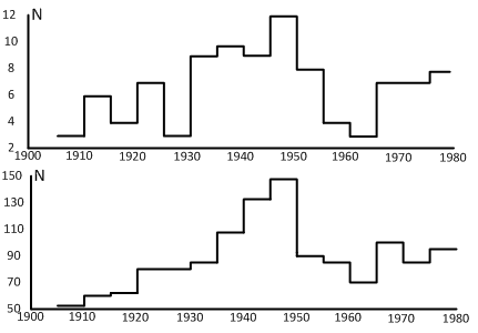
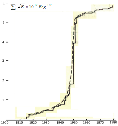
Several methods are being used for seismicity trend analysis. One method is to compare characteristics of seismic active period, include the lasting time duration, seismicity level (number of strong earthquakes, total released energy, etc.), and evolution characteristics of the seismicity process, etc; and predict the characteristics of future seismicity in the current seismic active period based on the comparison results. However, due to the limit of historic seismic data and the complexity of seismic process, features of different active period may show some repeatability but usually render distinct differences.

Another method is to apply seismic related and triggering factors in different seismic zones and belts. For example, the changing of the Earth’s rotation speed and sunspot activity level may induce the seismic activity. Fig. 1 clearly shows that the seismicity in China synchronizes with the global seismicity. Therefore the seismicity in mainland of China can be inferred from the global seismicity. Fig. 2 explains that when the Earth rotates faster, the activity of shallow earthquakes in North China-Northeast Plain usually decreases, while the seismicity in the regions of Liupan mountain-Qilian mountain-Altyn mountain increases, and vice versa. Thus, the seismicity level in those areas can be predicted from the variation of the Earth’s rotation speed.

The third method is based on characteristic analysis of the curves of released strain energy in seismic areas. The released strain energy curves can be classified to three types. (1) Linear type with stable slope, the corresponding seismic areas have comparatively high seismicity level, where strong earthquakes occur frequently with regular time interval. The maximum earthquake magnitude can be extrapolated from the curve (as shown in Fig. 3). (2) The curve with increasing slope, which indicates a high level of accumulated strain energy in corresponding seismic areas thereby indicating strong seismic activities in the future (Fig. 4). (3) The curve with decreasing slope, from which it can be deduced that the future seismicity level will not be too high in the corresponding seismic areas (Fig. 5).

Figure 1. Frequentness of earthquakes in global and mainland of China (a) Ms ≥ 63/4 shallow earthquakes in mainland of China (b) global earthquakes with Ms≥ 7

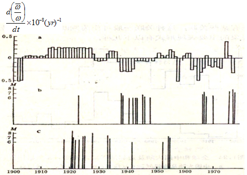Figure 2. (a) Rate of change of the Earth’s rotation angular speed (b) shallow earthquake in North China-Northeast Plain (c) earthquakes in Liupan-Qilian-Altyn

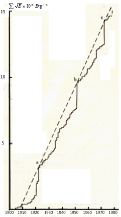Figure 3. Curve of released strain energy in Taiwan seismic zone

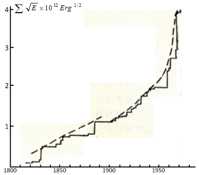Figure 4. Curve of released strain energy in North China seismic subzone

Figure 5. Curve of released strain energy in South Tibet seismic belt

Another type of method is mathematical statistics, which selects a character of the seismic activity (such as the magnitude, energy, time interval, etc.) and assumes that its data has some type of distribution (normal distribution, Gaussian distribution, Weibull distribution, etc.). The selected data is arranged into a series according to a certain order (magnitude order or chronological order, etc.), and fitted by a curve; the seismic trend then can be determined from interpolation or extrapolation of that curve. There are a number of methods that belong to the group of mathematical statistics method, such as maximum prediction, regression analysis, periodogram analysis, statistical prediction of stationary independent processes, wavelet analysis, entropy spectrum analysis, and so on. In applying those methods, there are two things need to be noticed: (1) the prediction results obtained from different methods may not be identical and even contradict each other, therefore we have to use different methods to obtain the results and find the average value as the final decision; (2) interpolation is superior to extrapolation because the latter can only predict one point at each time.

Among the presented methods, method 1 and 3 are main methods which are indispensible for seismicity trend analysis while method 2 and 4 are auxiliary methods. However, in current seismic safety evaluation, the seismicity trend is predicted based on mathematical statistics (method 4). Even worse, in using mathematical statistics to predict the future seismicity trend, only periodogram analysis is being used where five extra points are extrapolated from current periodogram to predict the seismicity trend in next 50 years. The prediction made using this method obviously underestimated the potential seismic risk, sometimes is inconsistent with the real situations of historic and contemporary seismic activity, and may be in disagreement with the zonation of the potential seismic source area. Fortunately, the seismicity trend analysis results did not affect the results of seismic hazard assessment because the zonation of the potential seismic source area is appropriate and various factors that affect the seismic hazard assessment have been fully considered. In deciding the seismicity parameters, the α value of the central area was increased to 11.35, thus, the ground motion parameters and conclusions made in current seismic evaluation reports of Shanghai are reliable and safe enough.

3. Working Procedure

(1) Select appropriate area for study. In this step, we need to select an entire seismic active area, neither choose part of that area nor mix one seismic active area with another. If the selected area is not appropriate for seismic study, it will be difficult to obtain regular historic statistical law from the study, therefore fail to provide meaningful historic data for seismicity trend analysis.

(2) Investigate the seismicity in different seismic periods by making diagrams of M-t, , and N-t. Plot the distribution of epicenter in different seismic periods to study the spatial evolving process of the seismic activity. Important factors that affect the spatial evolving process include: (a) if those seismic periods appeared regularly, the duration of each seismic period, their seismicity level, and similarities and differences among the seismic activities in different periods; (b) characteristics of the spatial distribution of different seismic periods; (c) correlations (especially the sequential relationship) among seismic activities in different seismic zones and belts, and epicenter migration; (d) effects of some environmental factors (rotation of the Earth, sunspot, tides, etc.).

(3) Determine the current stage of the seismic activities and predict the future seismicity level. For example, the seismicity in a seismic zone will be in active period in the near future if one of following conditions is satisfied. (a) The seismicity is in an active period and its lasting time is shorter than the shortest active period in history; (b) it is in a quiet period but its lasting time is close to the longest quiet period in history; or (c) the strain release curve accelerates.

(4) Determine and predict the intensity of seismic activity using extrapolation of the strain release curve or the data obtained from mathematical statistics.

(5) Roughly estimate the risk zones of strong earthquakes, major seismic active areas in current stage, epicenter migration, immunity zones of strong earthquakes, and intervals of time in which strong earthquakes occur.

Fig.6 displays the flowchart of trend analysis of seismicity.

Figure 6. Flowchart of trend analysis of seismicity

Table 1. Conserving probabilities of historical seismic data in Eastern China Century 1 2 3 4 5 6 7 8 9 10 Conserving probability 0.05 0.06 0.05 0.05 0.06 0.07 0.08 0.08 0.07 0.08 Century 11 12 13 14 15 16 17 18 19 20 Conserving probability 0.18 0.37 0.55 0.73 0.91 1.00 0.87 0.96 1.00 1.00

4. Seismicity Trend in Interested Areas

4.1. Data

The study area of this research, the seismic zone from lower reaches of YangtzeRiver to southern Yellow Sea, includes two areas: Eastern China (29º-37º N, 100º-124º E) and Shanghai and its vicinity (29º-34º N, 118º-124º E). All the historical seismic data of these two areas used for this study come from local historical records (for earthquakes occurred before 20^th century) and seismic data recorded by local observatories (for earthquakes occurred since 20^th century, especially since last 70’s) [1-3]. Lee et al. [4] studied the conserving probability of seismic data in Eastern China based on completeness of the historical records and obtained the conserving probabilities of Eastern Chinese seismic data in different centuries (Table 1). From Table 1, it can be found that a complete historical catalog (with probability close to 1) of Eastern Chinese earthquakes is only available after 15^th or 16^th century (after 1400 or 1500), which can be used for statistical analysis.

Based on all available historical seismic data, it can be concluded that: (1) historical records for earthquakes occurred in that area before 1491 are seriously missed. (2) From 1491 till 1900, the records for land and coastal earthquakes with Ms ≥ 5.0 are fairly complete, but most sea earthquakes were not recorded except four sea earthquakes with Ms ≥ 6.7. (3) Since 1905, with application of modern monitoring instruments, a complete seismic data of all the earthquakes with Ms ≥ 5.0 in this area becomes available. Hence, in this research we investigate the seismic data of earthquakes with Ms ≥ 5.0 which occurred after 1491 and especially focus on those occurred since 1905.

4.2. Comparison of Active Periods

Following figures and tables compare the characteristics of earthquakes occurred in the Y-Y seismic zone during different episodes since 1491.

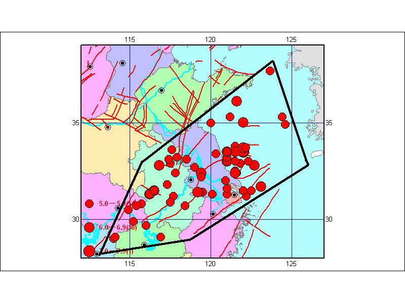Figure 7. Distribution of epicenters of earthquakes in Y-Y zone (1491-1998, Ms ≥ 5)

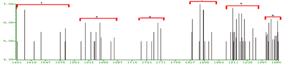Figure 8. M-T plot for historical earthquakes in Y-Y zone (1491-1998)

Figure 9. M-T, N-T, and-T plots for earthquakes in the fifth episode (1897-1954).

Figure 10. Distribution of epicenters of earthquakes in (a) 1st episode (1491-1585) (b) 2nd episode (1615-1679) (c) 3rd episode (1731-1770) (d) 4th episode (1829-1868) (e) 5th episode (1897-1954) (f) 6th episode (1974-?).

Table 2. Main areas of seismic activity 1st episode 2nd episode 3rd episode 4th episode 5th episode 6th episode Main seismicity areas (with all earthquake groups larger than Ms6.0) Southern sag, Ms6.7 in 1505 Qinling-Dabie, Ms6.0 in 1652 Lower Yangtze, Ms6.0 1764 Southern sag, Ms7.0 in 1846, Ms6.7 in 1852, Ms6.7 and Ms6.2 in 1853 Northern sag, Ms6.8 in 1910, Ms6.2 in 1932 Southern sag, Ms6.2 in 1984 Qinling-Dabie Lower Yangtze, Ms6.0 in 1624 Qinling- Dabie Qinling-Dabie, Ms6.2 in 1831 Southern sag, Ms6.5 in 1921 and Ms6.5 in 1927 Offshore areas of Yangtze estuary, Ms6.1 in 1996 LowerYangtze Qinling-Dabie, Ms6.2 in 1917 Lower Yangtze, Ms6.0 in 1979 Lower Yangtze Northern sag

Table 3. Division of seismicity episodes in Y-Y seismic belt Episode 1(1491-1585) 2(1615-169) 3(1731-1770) 4(1829-1868) 5(1897-1954) 6 (1974-) Releaseperiod main residual main residual main residual main residual main residual Lasting period 1491-1537 1538- 1585 1615- 1654 1655- 1679 1731- 1770 1829- 1855 1856- 1868 1897- 1934 1935- 1954 1974- 1998 1999- Groups 47 48 40 25 N/A 27 13 38 20 25 N/A N5 4 3 8 2 6 7 2 14 3 13 3 N5/year 0.15 0.06 0.2 0.08 0.15 0.26 0.12 0.50 0.15 0.52 N/A ΔT5(mo) 182.7 N/A 66.6 N/A 93.6 51.8 N/A 25.8 N/A 23.7 N/A σ5 19.4 N/A 16.8 N/A 14.2 23.4 N/A 4.8 N/A 4.4 N/A 187/60.7 86.2/22.1 93.6/14.2 58.3/17.9 36.1/6.9 N/A ΔT5max 221 N/A 122 N/A 139 158 N/A 57 N/A 58 N/A N6 1 0 2 0 1 4 0 5 0 3 0 Mmax 6.7 5.7 6.0 5.2 6.0 7.0 5.5 6.8 5.7 6.2 5.5 Released energy (1013 J) 72.32 3.56 16.98 0.6 10.72 368.3 1.32 204.2 3.04 35.73 N/A Energy /year 1.54 0.07 0.42 0.024 0.26 13.6 0.10 6.81 0.15 1.43 ΔTmr5 (mo) 454 229 N/A 93 100 82 ΔTmr6 (mo) 379 23 N/A 31 19 15

4.3. Statistical Forecast of Seismicity in Subareas

Next, we divided the Y-Y belt into three subzones (north, central, and south) and the intensity of seismicity in the decades to come in those subzones were estimated using statistical forecast.

Figure 11. Distribution of earthquakes in Shanghai and its vicinity, as well as northern, central, and southern parts of this area

Figure 12. M-T plots for earthquakes in Shanghai and its vicinity, as well as northern, central, and southern parts of this area

Earthquake recurrence period TM can be decided as:

(1)

where m is time with the unit of year. Forecast results are displayed in Table 4.

Table 4. Forecast of earthquake recurrence period Area Forecast results Y-Y belt 50 years for Ms6.0 earthquakes and 100 years for Ms6.5 earthquakes North subzone Possibility of occurrence of Ms6.0 earthquakes in next 50 years Central subzone Possibility of occurrence of Ms5.2 earthquakes in next 50 years South subzone In the decades to come the seismicity level stays about Ms4.0

An alternative method to determine the earthquake recurrence period is the maximum entropy spectral analysis, whose maximum entropy power spectral density S(f) is:

(2)

In above equation, A_m,i is the filtration coefficient of predicting errors, P_m is the variance of parameter estimation based on the autoregressive model, m is the order of the power spectrum, and f_i is the autocorrelation function of the stationary process.The maximum entropy spectral analysis results are displayed in Table 5.

Table 5. Maximum entropy spectral analysis results Area Analysis results Y-Y belt Maximum earthquake that may occur in next 20 years is about Ms6.5 North subzone Possibility of occurrence of Ms5.5 earthquakes in next 10 ~ 20 years Central subzone In next 10 ~ 20 years the seismicity level stays about Ms6.0 South subzone In next 20 years the seismicity level varies between Ms3.0 ~ 4.0

The seismicity level in those areas can also be predicted through periodogram analysis of Fourier series. In such analysis, we use every 10 years as an interval, and the logarithm of the maximum released energy during each interval, logE, is used as a statistical data.Table 6 lists the prediction results.

Table 6. Periodogram analysis results using Fourier series Area Analysis results Y-Y belt Maximum earthquake of about Ms6.2 may occur in next 10 years North subzone Maximum earthquake of about Ms5.0 may occur in next 10 years Central subzone Maximum earthquake of about Ms6.2 may occur in next 20 years South subzone No >Ms5.0 earthquake will occur during next 20 years

Next, five statistical methods – fuzzy modular neural network (method 1), gray modeling method (method 2), extreme value theory (method 3), prediction method based on probability of distribution of time interval of strong earthquakes (method 4), and Weibull distribution of time interval of strong earthquakes (method 5) were applied to separately estimate the maximum magnitude of the earthquakes that will occur in the Y-Y seismic belt during next 50 and 100 years. Table 7 displays the estimated maximum earthquake magnitude.

5. Medium’s Q Value and Stress Drop of Partial Small-Medium Earthquakes in Y-Y Seismic Belt

5.1. Studied Area and Data

In order to reveal the relationship among earthquake magnitude, Q value, and stress drop of small earthquakes, the study area (29º~34ºN, 119º~124ºE) is divided into five small regions based on distributions of potential hypocentral regions and earthquakes so that each region possesses a certain amount of records of earthquake data (Fig. 13). Average Q value and stress drop Δσ are calculated for each region. Specifically, since the Ms6.1 occurred in Nov-9-1996 at (32ºN, 123ºE) had a evident influence on Shanghai are, the current Q values and Δσ are calculated as well as the then values before and right after that earthquake.

Table 7. Statistical estimation of maximum earthquake magnitude during the next 50 and 100 years in Y-Y seismic belt and its three subzones Area Method 1 Method 2 Method 3 Method 4 Method 5 Summary Y-Y seismic belt 50 years 6.6 7.0 ≥6.5 (58%) ≥6.0 (60%) ≥6.0 (77%) ≥6.0 (60%) 100 years 7.0 ≥6.5 (58%) ≥6.0 (85%) ≥6.0 (81%) ≥6.0 (85%) Northern part 50 years 6.5 7.0 ≥6.5 (56%) ≥6.0 (59%) ≥6.0 (75%) ≥6.0 (60%) 100 years 7.0 ≥6.5 (56%) ≥6.0 (84%) ≥6.0 (80%) ≥6.0 (80%) Central part 50 years 5.8 6.1 ≥6.2 (55%) ≥5.0 (78%) ≥5.5 (54%) ≥5.0 (78%) 100 years 6.1 ≥6.2 (55%) ≥5.5 (100%) ≥5.5 (68%) ≥5.5 (68%) Southern part 50 years 4.0 4.2 ≥4.0 (60%) ≥4.0 (60%) ≥3.5 (61%) ≥4.0 (60%) 100 years 4.8 ≥4.0 (60%) ≥4.0 (100%) ≥3.5 (67%) ≥4.0 (100%)

Figure 13. Partitioning of study area (a) five regions (b) potential hypocentralretions

Seismic data are selected from the records of Shanghai earthquake networks. Those clearly recorded and unclipped seismograms are selected. Magnitudes of selected earthquakes range from M_L2.0 ~ 4.0 and epicenter distances vary within 100 ~ 200km, aftershocks are excluded. Additionally, seven digital seismic records are selected, which were recorded by Shanghai digital earthquake network, which was put into operation in 2001. Thus, overall 92 earthquakes are used for our study.

5.2. Methods and Data Processing

Solve medium’s average Q values

Assume n earthquakes are recorded by an observatory within the same area and spectrum of the i^th earthquake is:

(3)

where A_i0(ω) is the seismic spectrum emitted from the hypocenter, G(R_i) is geometric diffusion, R_i is hypocentral distance, I(ω) is frequency characteristic of instruments, exp[-(ωR_i)/(2v_pQ)] is medium absorption, and v_p is the velocity of P-wave which takes the value 5.7km/s.

Substitute two fixed frequencies, ω₁ and ω₂, into above equation separately and make a division, we can have

(4)

where (ω₁ – ω₂)R_i/(2v_pQ) is a constant. Meanwhile, since our selected range of earthquake magnitude is comparatively small and those earthquakes occurred in the same region, therefore the Ln|A_i(ω₁)/A_i(ω₂)| of different earthquakes can also be regarded as a constant. Those assumptions transform Eqn. (4) to

(5)

In above equation, Y_i can be calculated, R_i is known, and coefficients a and b can be solved using least squares method. The average Q value of this region then can be solved from b as:

(6)

Solve stress drop Δσ

By using dislocation model of circular shear to simulate the medium and small strike-slip earthquakes and taking samples from the seismogram and then performing Fourier analysis, the source spectra can be obtained after taking off instrumental and medium effects. From that spectra the spectral amplitude in lower band u(ω)_ω→0 and corner frequency f_cα can be obtained, therefore the seismic moment m₀ can be determined from

(7)

where ρ is the medium’s density (we use 2.7 × 10³ kg/m³ for the crust), r is the hypocentral distance, the radiation pattern R_α = sin(2θ)cosΦ (if θ and Φ are unknowns, we can take the average radiation pattern calculated over the focal sphere, 4/15 for the P wave [8], and v_p means P-wave velocity (we assume v_p = 5.7km/s within the crust [9]). The radius of rupture circle a can be calculated from the corner frequency f_cα as:

(8)

In above equation, the rupture propagation velocity v_f = 0.775v_s, where v_s is S-wave velocity (we assume v_s = 3.38km/s within the crust [10]). Finally, the stress drop Δσ can be calculated using Eqn. (9) based on m₀ and a

(9)

Data processing

For the analogous records, they are scanned and digitized through the seismogram digitization and database management system (SDDMS) [11]. Through that system the sampling rate can be selected. Considering quality of the analogous records and range of interested corner frequency f_cα, the sampling rate is set as 200 dpi. Sampling step size Δt is set as 0.0635 seconds and the window length T is 6 seconds. For small earthquakes around M_L3.0, the variation range of the corner frequency is 2 ~ 4Hz. Therefore the window length of 6 seconds is 12 times as long as the reciprocal of minimum corner frequency (1/(f_cα)_min = 0/5seconds), which guarantees an enough frequency spectrum’s resolution. Meanwhile, the Δt of 0.0635 seconds is less than 1/(2(f_cα)_max = 0.125 seconds, so that the high-frequency aliasing can be prevented.

The digitized records and waveforms are then adjusted by the SDDMS system through slant correction, removing DC component of baseline, and arc correction. Afterwards, the Hanning window and fast Fourier transform (FFT) are applied to obtain the spectra of seismic waves. The average Q value of a selected region then can be solved using the method presented above. Also, based on the obtained spectra of seismic waves, the source spectra are obtained after instrument and medium calibration, and the stress drop Δσ can be solved using the method presented above. The Hanning window W(t) is

(10)

Characteristic of medium frequency B(ω) is

(11)

where we assumed the low cutoff frequency ω is 0.25.

For the digital records, their spectra of seismic waves can be directly obtained applying the Hanning window and FFT based on a sampling rate 100 dps. Because the digital seismometer is a broadband seismometer, the instrument calibration is not necessary and the source spectra can be obtained after the medium calibration.

5.3. Summary

The solved results are displayed in Fig. 14 and Table 8. The relative errors of spectral curves caused from digitalization are about 1~ 2% [12] and the errors of the Q values are in the same magnitude. Thus, the presented differences among the average Q values of different regions are meaningful. The most important factor that causes errors in stress values is the error of earthquake magnitude, whose maximum acceptable value is 0.3. The maximum relative error of stress τ₀ can reach 70% [12]. Since the average stress value of each region is a result of multiple earthquakes, it can be considered that the average stress drops in regions A, B, and C are comparatively higher, next are the stress drops in regions E and F, and the stress drop in region D is the lowest.

From the calculation results, it is observed that the highest average Q value appears in region A’s sea area, which is 412. Other high Q values include 348 which appears in the central Jiangsu Province and coastal area of region B; 340 which appears in region F (close to the epicenter of the Nov-9-1996 earthquake); and 305 which appears in Liyang of region C. The lowest average Q value appear in Shanghai and the sea area to the east of Hangzhou Bay (in region D), which is 241. And the Q values in other regions are 289. Comparing the distribution of Q values to the potential seismic source areas, it shows that the higher Q values appear in the potential source areas of higher-magnitude earthquakes. This is because that only under a high Q value, the medium can accumulate high-level stress therefore gives rise to strong earthquakes.

The Q value in region F dropped from 352 to 342 after the Ms6.1 earthquake occurred in Nov-9-1996 on estuary of Yangtze River. Normally, the Q value will drop after the mid-strong earthquakes because of destruction of local medium. Considering measurement errors, the decrease in Q value after that Ms6.1 earthquake is slight, which indicates that the damage caused by the Ms6.1 earthquake in the local medium was small. The current Q value in that area is 340, which is the same as the one right after the Ms6.1 earthquake.

From distribution of the stress drop Δσ, it is found that the drop is high in regions A, B, C, and the next high Δσ appears in regions E and F. The stress drop in region D is comparatively low. From time evolution, it seems that the period of high stress drop corresponds to the time period of high seismicity level in that region.

Based on above discussion, it should be noted the possibility of about Ms6.0 earthquakes in the Southern Yellow Sea and coastal area (regions A and B), the sea area to the east of Yangtze estuary (region F) and Liyang and vicinity (region C).

Table 8. Q values and stress drop Δσ of small earthquakes in lower reaches of Yangtze River – Yellow Sea seismic belt Region Avg. Q and Δσ Origin time Location of epicenter ML Δσ (bar) A Q = 412Δσ = 1.34bar 1975.06.08, 11:02 32°17' 121°49' 3.9 7.05 1979.02.16, 14:57 33°48' 122°12' 3.5 2.21 1979.04.16, 18:49 32°52' 121°41' 3.6 0.86 1979.04.25, 02:43 33°23' 122°49' 3.5 0.26 1979.04.28, 09:15 32°53' 121°27' 3.0 0.19 1980.04.14, 22:57 32°36' 122°32' 3.1 0.80 1980.06.01, 18:59 32°36' 123°24' 3.3 1.75 1992.03.22, 16:57 34°20' 122°06' 2.7 0.004 1997.07.28, 03:36 33°43' 122°14' 2.9 0.226 1999.02.15, 11:21 32°48' 123°30' 2.9 0.082 B Q = 348Δσ = 1.11bar 1978.07.06, 11:44 32°43' 120°57' 3.7 1.66 1979.01.04, 18:28 33°50' 120°33' 4.3 3.04 1983.09.25, 14:30 32°50' 120°49' 3.1 0.60 1983.10.19, 14:25 32°51' 120°07' 3.5 0.24 1984.04.22, 19:25 33°49' 121°25' 4.1 0.17 1984.05.16, 17:16 33°35' 120°35' 3.6 1.99 1984.05.17, 11:59 33°05' 120°31' 3.5 0.79 1985.04.04, 08:24 32°53' 120°19' 3.3 0.19 1985.05.13, 03:48 32°46' 120°43' 4.1 1.35 1990.04.19, 06:00 33°19' 121°01' 2.8 4.0 1992.01.27, 19:34 32°40' 120°22' 2.5 0.014 1996.07.28, 14:58 33°44' 121°07' 2.9 1.42 1998.03.31, 23:24 33°32' 120°38' 2.7 0.058 1999.05.29, 15:16 33°20' 119°56' 2.6 0.050 C Q = 305Δσ = 0.917bar 1979.03.07, 05:08 30°45' 119°19' 3.9 1.17 1979.07.09, 22:13 31°26' 119°14' 4.2 2.94 1979.07.11, 03:08 31°26' 119°16' 3.4 0.49 1979.07.15, 14:28 31°26' 119°16' 2.7 1.14 1979.07.16, 10:41 31°27' 119°16' 2.7 0.37 1979.07.22, 03:12 31°26' 119°18' 3.5 2.39 1979.07.23, 12:38 31°27' 119°19' 2.6 0.28 1979.07.26, 07:33 31°26' 119°17' 3.2 0.12 1979.07.27, 07:11 31°27' 119°17' 3.2 0.98 1979.07.29, 10:21 31°27' 119°17' 2.8 1.52 1981.03.25, 06:35 31°25' 119°17' 3.9 1.0 1981.11.18, 20:36 31°17' 120°12' 2.8 0.20 1982.03.29, 19:40 31°28' 119°17' 4.1 5.0 1982.04.08, 21:26 31°29' 119°17' 3.8 0.33 1983.08.10, 18:09 31°26' 119°17' 2.8 0.96 1984.04.30, 12:48 31°22' 119°14' 3.6 1.15 1984.06.01, 09:24 32°00' 119°26' 3.0 0.51 1985.07.14, 01:51 31°26' 119°28' 2.6 0.25 1996.04.07, 00:53 32°31' 119°36' 2.6 0.029 1996.04.07, 01:47 30°56' 119°01' 2.9 0.042 2001.08.10, 16:51 30°44' 119°05' 2.5 0.029 2001.10.17, 11:57 31°53' 119°18' 2.8 0.101 2001.10.18, 15:25 31°04' 119°37' 2.8 0.101 D Q = 241Δσ = 0.286bar 1975.12.31, 06:35 30°06' 121°54' 2.4 0.56 1978.03.05, 14:40 31°30' 123°36' 2.9 0.91 1978.11.15, 12:41 30°18' 122°30' 2.5 0.19 1982.03.23, 02:53 31°17' 123°19' 3.3 0.70 1992.06.24, 19:33 31°30' 122°00' 2.7 0.028 1992.10.08, 05:13 31°00' 121°21' 2.8 0.058 1995.04.02, 08:20 31°12' 121°25' 2.9 0.064 1996.05.28, 09:16 30°26' 121°47' 2.4 0.025 1996.10.20, 17:00 31°06' 123°32' 2.9 0.042 E Q = 289Δσ = 0.487bar 1975.10.07, 21:10 30°06' 123°03' 3.4 0.23 1976.01.10, 05:08 29°55' 122°50' 3.5 0.56 1978.02.12, 05:30 33°09' 118°34' 3.4 0.36 1978.06.02, 16:51 30°52' 120°51' 2.3 0.16 1978.06.16, 03:09 33°55' 118°02' 3.8 1.35 1978.11.27, 11:50 32°07' 121°42' 3.1 0.98 1983.07.03, 23:21 31°55' 120°45' 3.3 1.60 1984.06.25, 23:35 30°36' 119°52' 2.9 0.52 1984.07.06, 12:55 29°51' 121°23' 2.8 0.43 1985.01.06, 03:42 31°07' 120°31' 3.2 0.25 1985.05.02, 20:36 31°53' 120°36' 3.3 2.54 1985.06.01, 21:18 31°16' 120°23' 2.6 0.33 1990.05.31, 04:18 31°36' 120°28' 2.9 0.082 1993.02.02, 21:41 29°37' 120°00' 2.3 0.012 1993.09.04, 20:59 29°41' 121°36' 2.4 0.018 1997.08.19, 00:08 32°01' 123°14' 2.8 0.101 1997.12.18, 12:14 32°11' 123°14' 2.8 0.030 1998.06.02, 20:18 29°30' 120°48' 2.6 0.029 1998.10.14, 14:30 30°03' 120°47' 2.9 0.082 2001.11.27, 01:04 31°53' 123°22' 2.8 0.082 F Q = 352Δσ = 0.170bar 1981.03.30, 07:22 31°32' 123°34' 2.7 0.021 1982.05.27, 08:06 31°30' 122°54' 2.5 0.036 1990.03.06, 07:43 31°29' 123°32' 3.3 0.328 1994.03.18, 22:15 31°44' 122°55' 2.6 0.234 1995.07.05, 11:58 31°28' 123°35' 3.2 0.232 Q = 342Δσ = 0.403bar 1996.11.09, 22:08 31°54' 123°06' 3.9 1.333 1996.11.18, 15:51 31°41' 123°23' 3.3 0.071 1996.11.20, 20:19 31°53' 123°09' 3.5 0.244 1996.12.02, 01:50 31°53' 123°17' 3.2 0.119 1996.12.06, 22:03 31°53' 123°18' 3.1 0.084 1996.12.06, 22:14 31°55' 123°12' 3.3 0.567 Q = 340Δσ = 0.573bar 1998.01.03, 19:34 31°53' 123°21' 3.5 0.244 1998.01.03, 19:41 31°53' 123°19' 3.0 0.931 1999.07.03, 18:16 31°58' 123°14' 3.6 1.597 1999.07.21, 10:57 31°52' 123°24' 2.8 0.030 1999.09.16, 17:26 31°42' 123°27' 2.9 0.064

Figure 14. Q values and stress drop Δσ in several areas in Shanghai and vicinity

6. Conclusions

The conclusions made based on the earthquake prediction can be listed as:

(1) Historical earthquakes occurred in the Y-Y seismic zone can be classified into six episodes and each episode can be divided into the main release period and the residual release period. The seismic activity level during the main periods is much higher than that during the residual periods and all earthquakes with Ms ≥ 6.0 occurred in the main release periods. The earthquake occurrence shows an obvious pseudo-periodicity during the main release periods. The duration of a main period is about twice as long as that of the residual release period.

(2) The criteria that indicates the transition from a main release period to a residual release period is: 1) the time interval between the last Ms ≥ 5.0 earthquake during the main release period and the first Ms ≥ 5.0 earthquake of the following residual release period is much longer than the maximum time interval of the Ms ≥ 5.0 earthquakes occurred during the main period; 2) an Ms ≥ 6.0 earthquake may occur about two years before the last Ms ≥ 5.0 earthquake of the main period.

(3) The Y-Y seismic zone is divided into four areas: the sea area of northern sag to the north of 35ºN, the sea area of southern sag to the south of 34ºN and the offshore area of Yangtze estuary, lower Yangtze block to the east of Tanlu fault (PTLF), and Qinling-Dabie block. The seismic activity level in the sea areas is higher than that on the lands and the highest seismicity level is in the sea areas to the south of 34ºN. Except for the current episode, Ms ≥ 5.0 earthquakes have occurred in all four areas during previous episodes.

(4) The current episode, which starts from 1974, likely entered into its residual release period in 1999. That period will end till 2012 and then enter into a seismically quiet episode. During this period, there may have two or three groups of earthquake with Ms ≥ 5.0, but the maximum magnitude will be lower than Ms6.0. According to the possibility order of the occurrence of future mid-strong earthquakes, the four areas can be arranged as: the sea area of southern sag to the south of 34ºN, the lower Yangtze block, the sea area of northern sag to the north of 35ºN, and the Qinling-Dabie block (from high to low).

Finally, based on all above work, we determine three seismic risk zones where mid-strong earthquakeswhich will cause damages may occur within the next 10 years. Those risk zones are: 1) southern sags of Southern Yellow sea and coastal regions, Ms ≥ 6; 2) Yangtze estuary and sea area to the east of it, Ms ≥ 5; 3) Changshu-Taicangarea, Ms ≥ 5 (Fig. 15).

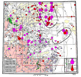Figure 15. Seismic risk zones