Abdullahi S. B. Gimba1, Luqman B. Umdagas2, Abdu Zubairu2, Velisa Vesovic3, Khadija S. Ibrahim1, Ikechukwu Okafor1
1Department of Petroleum and Gas Engineering, Nile University of Nigeria, Abuja Nigeria
2Department of Chemical Engineering, University of Maiduguri, Borno State, Nigeria
3Department of Earth Science and Engineering, Imperial College London, United Kingdom
Correspondence to: Abdu Zubairu, Department of Chemical Engineering, University of Maiduguri, Borno State, Nigeria.
| Email: |  |
Copyright © 2022 The Author(s). Published by Scientific & Academic Publishing.
This work is licensed under the Creative Commons Attribution International License (CC BY).
http://creativecommons.org/licenses/by/4.0/

Abstract
Natural Gas (NG) is receiving increased attention as world energy source due to its low environmental impact compared with other fossil fuels. NG is commonly shipped between continents as super-cooled liquid known as Liquefied Natural Gas (LNG). In over forty years of LNG shipping between continents, no carrier has experienced a total loss of containment. Notwithstanding, it is paramount to understand and predict the consequence of a spill either due to accidental spillage or deliberate sabotage. Several models have been developed that describe the LNG spill scenario both on land and water. Spills on water generally result in larger pools than land spills because they are mostly unconfined. Modeling of LNG spills on water is inherently difficult because the phenomena is very complex and the experimental basis is acutely limited. The complexity is particularly apparent when estimating the evaporation rate of LNG released on water. Most of the proposed models are hugely simplified, for instance, many overlook the influence of turbulence effects; consequently, unable to adequately capture real-life scenarios. In this work, we proposed a model that describes LNG spill on water that also accounts for the effects of turbulence. Simulation studies of LNG (50,000 kg) indicates a maximum pool radius of 80m in 95 seconds assuming ‘calm’ conditions; while the pool completely vaporized in 125 seconds, corresponding to a heat transfer coefficient of 465 W/m2K. Considering the turbulence effects, the pool vaporized in 60 seconds and heat transfer coefficient of 215 W/m2K, indicating about 50% overestimation of vaporization time. In the model validation, an average of 10% deviation in LNG mass boil-off of our simulation from experimental data was obtained, thus signifying a good agreement between the simulation and experimental data.
Keywords:
LNG, Heat Transfer Coefficient, Pool Boiling, Turbulence, Solar cell
Cite this paper: Abdullahi S. B. Gimba, Luqman B. Umdagas, Abdu Zubairu, Velisa Vesovic, Khadija S. Ibrahim, Ikechukwu Okafor, Modelling LNG Spill on Water: Effects of Turbulence, Frontiers in Science, Vol. 12 No. 1, 2022, pp. 1-8. doi: 10.5923/j.fs.20221201.01.
1. Introduction
Liquefied natural gas (LNG) is simply natural gas (NG) that is cooled to its liquid form at atmospheric pressure and temperature of about -162.2°C. LNG commonly consists of 85%-98% methane with the remainder being a combination of nitrogen, carbon dioxide, ethane, propane, and other heavier hydrocarbon gases [1]. The liquefaction process reduces the volume of the gas by nearly 600 folds. Due to its flammability, LNG possesses some hazardous properties. LNG is an efficient means of transporting natural gas to distant markets, not supplied by gas grid, connecting the extraction/production point to the users. Basically, the LNG process is composed of the following steps: extracted natural gas is liquefied in the production field or in a close site, after removing the impurities. Then, the LNG is loaded onto double-hulled ships which are used for both safety and insulating purposes and transported to the receiving harbour. As arrived, the LNG is loaded into well-insulated tanks and then, re-gasified in specific plants. At the end, the re-gasified natural gas is fed to the pipeline distribution system and delivered to the end-users. But, the high production, transportation and storage costs have reduced the LNG technology spread to specific cases in which there are no other cheaper ways to transport the gas. When LNG is spilled on water, it will vigorously boil and produce vapour cloud that will disperse. And if that vapour cloud is within its flammable range, it might ignite and cause explosions and or fires. The risks associated with the occurrence of such events (like loss of containment of storage tank or LNG carrier) need to be studied in order to determine the effects it might have on human and aquatic lives, facility, and the public at large [1]. Several models have been developed that describe the LNG spill scenario both on land and water [1-5]. Mathematically describing the whole processes involved in an LNG spill on water is very difficult. Therefore, for the purpose of modelling, some essential assumptions need to be drawn that will allow mathematical description of the fundamental features of an LNG pool after spill. In this work, we proposed a model that describes LNG spill on water that also accounts for the effects of turbulence.
2. Theory
2.1. Natural Gas
Natural gas is comprised primarily of methane with up to about 10% ethane and lesser quantities of nitrogen, propane, and higher aliphatic hydrocarbons (Figure 1). The boiling temperature at one bar is in the range of 111 K (depending upon composition) and the density is about 420-470 kg/m3 [2]. When natural gas is produced from the earth, it includes many other molecules, like ethane (used for manufacturing), propane (which we commonly used for backyard grills) and butane (used in lighters). We can find natural gas in Nigeria and around the world by exploring for it in the earth’s crust and then drilling wells to produce it. The composition of natural gas varies considerably depending on the origin of the gas and geographical location, as well as geological structure of the gas reserve [3].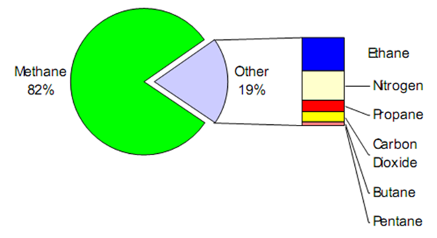 | Figure 1. Typical Natural Gas Composition [3] |
2.2. Liquefied Natural Gas
Liquefied natural gas (LNG) is natural gas that has been cooled to the point that it condenses to a liquid, which occurs at a temperature of approximately -256°F (-161°C) and at atmospheric pressure through a complex cryogenic process called liquefaction. Liquefaction reduces the volume by approximately 600 times thus making it more economical to transport between continents in specially designed ocean vessels, whereas traditional pipeline transportation systems would be less economically attractive and could be technically or politically infeasible. Figure 2 illustrates the economic advantage of LNG transport over other options.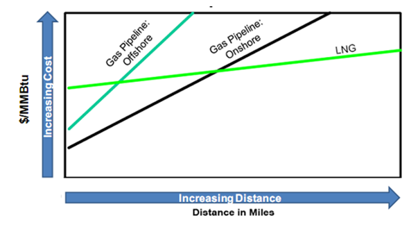 | Figure 2. Natural gas transportation costs, modified from [3] |
Upon delivery to a final destination the LNG is pumped into either another cryogenic storage facility or is channelled to a regasification unit where it is vaporized back to gaseous form, and subsequently pumped through pipeline system that leads to an ultimate market, as illustrated in the LNG value chain in Figure 3. Thus, LNG technology makes natural gas available throughout the world [4]. Currently, imported LNG is commonly 95% – 97% methane, with the remainder a combination of ethane, propane, and other heavier gases and it varies with location around the globe [5]. LNG vapour is colourless, odourless, and non-toxic, and is considered flammable. LNG vapour typically appears as a visible white cloud, because its cold temperature condenses water vapour present in the atmosphere. The lower and upper flammability limits of methane are 5.5% and 14% by volume at a temperature of 25°C [6].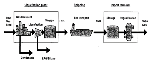 | Figure 3. LNG process value chain [3] |
3. Materials and Method
The fundamental processes involved in an LNG spill on water are: (1) Pool spreading (2) Pool vaporization (3) Heat transfer from the underlying water (heating source) to the LNG pool. Other processes like water entrainment and hydrate formation as well as heating source from the surrounding air are neglected in this study. Therefore, heat transfer was assumed to be wholly from the water over which the LNG spreads.
3.1. Pool Spreading
The adopted models for pool spreading were generated while assuming a circular liquid pool of radius (r) and radial liquid flow velocity on water [7] as illustrated in Figure 4 (a). The flow was assumed to be in gravity-inertia regime while the inertial forces control; and a resistance term corresponding to friction at the bottom of the pool [8]. Gravity-viscous or surface tension-viscous regimes are assumed negligible throughout the duration of the pool spread because the LNG rapidly vaporizes before other regimes become noticeable [1]. The force needed for radial acceleration of the cryogen was provided by the pressure head. Moreover, sea currents and waves action, preferential boiling and pool break-up are also neglected [7].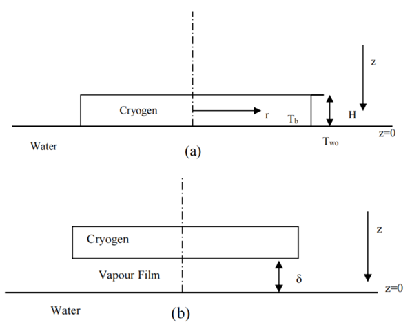 | Figure 4. Model of heat transfer to LNG boiling on water (a) start of boil-off (b) on set of film boiling [3] |
Instantaneous spill from point source was assumed. Though, some researchers debated that an instantaneous release scenario is unrealistic even for huge tank rupture sizes. Notwithstanding, this assumption is undoubtedly true particularly in the case when the release time is negligible compared to the spreading time [3]. LNG was modelled as pure liquid methane, which upon release, was assumed to be at its boiling point, the pressure was assumed atmospheric, and water temperature was assumed to be 293K through out the period of vaporization, as the unconfined body of water is considerably large with adequate mixing, hence sufficient amount of heat is supplied to the cryogen. The amount of LNG released is 50,000 kg.The model for pool spreading during an LNG spill on water includes a relative density term showing that the LNG layer displaces the water downward to some extent as expressed in Equation 1 [8]. 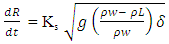 | (1) |
Where R is the pool radius (m), t is the time (s), Ks the spreading constant, g is the gravitational acceleration (m/s2), ρw is the water density (kg/m3), ρL is the density of liquid LNG (kg/m3) and δ is the thickness of LNG layer (m).The value of the spreading constant in Equation (1) is usually computed from experimental results. Values from 1.77 to 4.0 have been reported in the literature. A theoretical value of 1.16 was suggested by [8], but argued that in order to achieve a more accurate result in matching experimental data, higher value is recommended. Ks value of 1.41 is the most commonly suggested. A similar spreading equation to Equation (1) was reported in [3] and [9] with spreading constant values of 2.69, and 1.64 respectively. In this work, however, 1.64 was used.
3.2. Pool Vaporization
In order to determine the rate of liquid vaporization, it was assumed that the main heating source was solely the water over which the LNG spreads. Other sources of heat (i.e., surrounding air) was neglected. It was also assumed that, upon release, the LNG instantaneously reaches its saturation temperature, thus overlooking any sensible heat gain. All heat transferred to the LNG was assumed to be entirely used for vaporization. With these assumptions, the equation for LNG pool vaporization rate adopted from [3] was expressed by a first order differential equation given by Equation (2):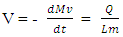 | (2) |
where V is the vaporization rate, Mv is the mass of liquid vaporized, and LM is the latent heat of vaporization of LNG. Q is the total heat flow to the LNG pool, expressed as the product of the heat flux q and the heat transfer area A.Upon release, as LNG pool is undergoing spreading, its radius, R, increases with time (Equation 1). Hence, the vaporization equation (Equation 2) is coupled to the spreading equation (Equation 1). The two first order differential equations were solved under the following boundary conditions: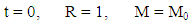
3.3. Heat Flux
The heat flow to the LNG pool across the water cryogen boundary can be expressed with a convective heat equation: 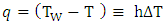 | (3) |
where T and TW (K) are the temperatures of LNG and water respectively, h is the heat transfer coefficient (W/m2/K).The surface water temperature was assumed constant and no freezing of water surface. The boiling regimes will determine the heat flux into the pool. For nucleate boiling, the critical heat flux and critical temperature can be estimated using Equations (4) and (5) respectively proposed by Conrado & Vesovic [10]. | (4) |
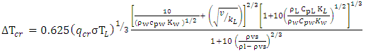 | (5) |
The minimum heat flux and temperature indicating the transition to film boiling regime can also be estimated using the Equation (6) adopted from [11].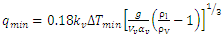 | (6) |
The correlation provided by [12] was used to determine the heat flux into the pool during the film boiling (see Figure 4 (b):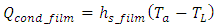 | (7) |
3.4. Heat Transfer Coefficient
For heat transfer coefficient, equation (8) suggested by [12] was used. | (8) |
where λv is the thermal conductivity of the cryogen vapour film at the film temperature (usually taken as the average of cryogen and water temperatures), Nu is the Nusselt number for film boiling and lc is the critical wavelength of instability obtained from equation (9).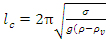 | (9) |
where ρ and ρv, are the densities of cryogen liquid and vapour respectively; σ is the interfacial tension between cryogen liquid and vapour, and g is the acceleration due to gravity. The equations for heat transfer coefficients for transitional and nucleate regions were adopted from [3].
3.5. Turbulence Factor
The actual heat transfer coefficient between the water and LNG, h; could be expressed in terms of the quiescent values given by Equation (10): | (10) |
Where h is the heat transfer coefficient derived from standard correlations for quiescent conditions [12]. The coefficient FT is defined as the turbulence factor, and is reliant on the cryogen spill area in addition to the cryogen contact velocity at the water surface. The turbulence factor defines the extent of agitation produced as a result of falling of the cryogen from the discharge height. The inertia that the cryogen landed with onto the water surface causes it to infiltrate the water level and causes significant mixing.To estimate the turbulence factor, correlations developed by [8] were used expressed as Equation (11):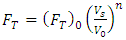 | (11) |
where FT is the turbulence factor, Vs is the cryogen velocity at the water surface, Vo is the reference cryogen velocity at the water surface and (FT)0 is the turbulence factor at reference spill velocity, and n is a velocity exponent which is a function of the discharge area. An alternative expression to Equation (11) in terms of volumetric flow spill rates is given as Equation (12).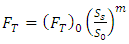 | (12) |
where Ss is the cryogen volumetric spill rate, So is the reference cryogen spill rate given as 0.292 and 0.150 m3/s for Esso-11 and Esso-12 tests respectively. While m is the spill rate exponent equals 0.2.The velocity with which the LNG reaches the water surface Vs in Equation (10) is the sum of the velocities at the discharge point (VD) and the velocity of free fall to the water surface. The latter could be derived by energy balance of the falling cryogen mass. The LNG velocity at the water surface is therefore given by Equation (13):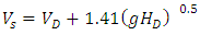 | (13) |
Where VD is the LNG velocity at discharge point and HD is the height of discharge point above water surface. To obtain the turbulence factor at the reference spill velocity (FT)0.
4. Results and Discussion
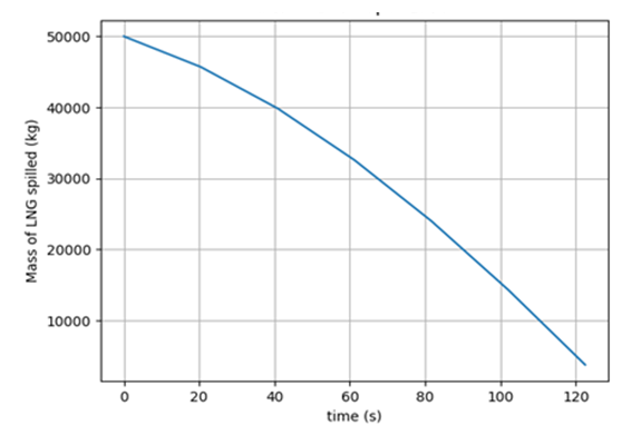
It could be seen from the spreading profiles in Figure 5 that when 50,000 kg of LNG is spilled on water surface, the radius continues to increases until it reaches a maximum at about 95 s corresponding to a radius of 80 m. Simultaneously with the pool spreading, the spilled cryogen undergoes boiling and vaporization processes due to the heat transfer from the underlying water. Consequently, the amount of the cryogen spilled continues to decrease until it has all vaporized in about 120 s as shown on the vaporization rate profile in Figure 6. This, while neglecting all external disturbances, like the effects of wind current and wave actions. Furthermore, the turbulence effects were also neglected here. The result obtained here was in congruence with the works of [10] and [13]; the former spilled 50,000 kg and the latter spilled 70,000 kg of liquid methane, the liquid pool completely vaporized in about 120 seconds and 170 s respectively.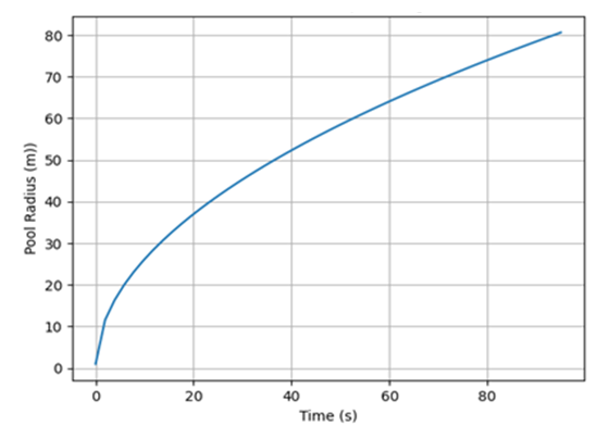 | Figure 5. Rate of LNG pool spreading |
 | Figure 6. Rate of LNG pool vaporization |
4.1. Heat Transfer Coefficient
The heat transfer coefficient was estimated at approximately 155 W/m2 with a corresponding heat flux value of 28,000 W/m2.In conformance with the experimental observations of [2] and [14] in this model, the cryogen was allowed to boil through the three regimes for confined spills. Usually, confined spill scenarios match up with bench-scale laboratory experiments where the data used in this work was obtained.The heat transfer coefficient in the film boiling regime gave a value of approximately 150 W/m2s for pure liquid methane. Guerra [15] mentioned that the heat transfer coefficient for film regime calculated using Equation (8), resulted in boil-off times which are 300% higher than their pragmatic experimental values.
4.2. Turbulence Effects
The simulation in this work was conducted using the experimental conditions of Valencia-Chavez [2]: R-44 (M0 = 0.09kg, T0 = 285K) R-46 (Mo = 0.36322kg, To = 288K) and R-47 (Mo = 0.2445 kg, To = 284K) while incorporating the appropriate turbulence factor calculated for each of the runs such that the heat transfer coefficient, h, was computed. Thus, the heat transfer coefficient, h in the film boiling regime was obtained by multiplying the theoretical heat transfer coefficient presented by Equation (8) and the turbulence factor, giving a value of h = 465 W/m2K for film boiling and of h = 200 W/m2/K for transition boiling. Figure 7 compares the simulation results using the turbulence factors with the experimental values of Valencia-Chavez [2].The comparison of the mass vaporised shown in Figure 7 shows good agreement between the numerical simulation and the experimental values for all runs. The maximum deviations of the simulations results obtained compared to the experimental results were 7.0%, 10% and 12% for R-47, R-46 and R-44 respectively.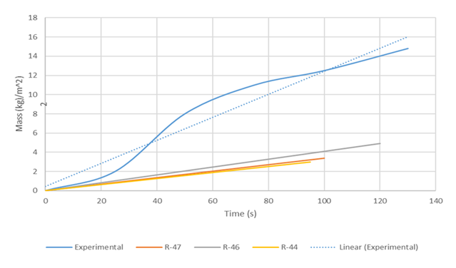 | Figure 7. Comparison of simulation runs using turbulence factors with Valencia-Chavez [2] experimental data |
The model was again used to simulatee conditions shown in Figure 5 and 6 which did not consider the effects of turbulence, and was compared with simulation incorporating the turbulence in runs R-46, R-47, R-6 [2]. It can be seen from Figure 8 that considering the effects of turbulence, for R-46, the cryogen pool evaporated in 40 s, giving about 200% overestimation of evaporation time if turbulence affects were neglected (120 s). Similarly, for both R-6 and R-47, the pool evaporated in about 60 s, giving about 100% overestimation of evaporation time for both runs.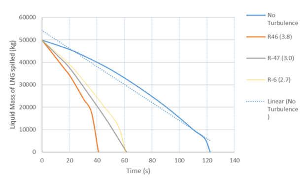 | Figure 8. Turbulence factors for Valencia Chavez experimental runs |
4.3. Model Validation
Laboratory experimental data reported by Boe [16], and Valencia-Chavez [2], were used to validate the model, because they were perceived comprehensive enough and provide the desired information. Besides, these data were precisely for experiments where LNG was modelled as pure methane analogous to the baseline assumptions in this work, hence providing a good basis for comparison.
4.3.1. Comparison with Valencia Chavez’s Experiment
The results of the model simulation of this work that accounts for effects of turbulence was compared with the experimental values from [2]. The experimental values tremendously uunderestimates mass boil-off compared to the numerical simulation of this work as can be seen from Figure 9. 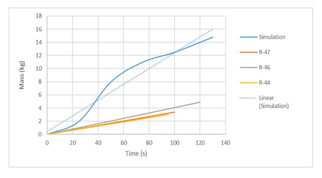 | Figure 9. Comparison of simulation with Valencia-Chavez [2] Experiment |
This can be attributed to the fact that the equations used to determine the heat transfer coefficient are in quiescent conditions and as such the heat flux reaching the water surface was low. Consequently, that under underestimates the heat transfer to the LNG pool. It can also be looked from the perspective of Valencia Chavez’s [2] experimental setup that turbulence effects were reduced, but notwithstanding, not wholly dampened. As the spill was considered instantaneous considering the spill time of about 1-2 seconds, the large initial mass of cryogen spilled will inevitably cause turbulence at impact with the water surface. Furthermore, another reason for the overestimation of mass boil-off time in his experimental run can be attributed to overlooking the impacts of turbulence effects.
4.3.2. Comparison with Boe’s Experiment
Boe’s [16] experiment is similar to that of Valencia Chavez [2], in that both made significant efforts to eliminate turbulence effects. The average spill time of the experimental series is 1.5 s. In the present work, two of Boe's experimental runs were selected: LCH-13 (Mo = 0.29 kg To = 298K) and LCH-15 (Mo = 0.28 kg, To = 314); which are fairly analogous to Valencia-Chavez's [2] runs that was simulated in terms of the amount of cryogen spilled, but only differ with higher initial water temperatures of 298 K and 313.5 K respectively. The two selected experimental runs were simulated using the resultant turbulence factors, and the results were then compared with the experimental values. Both experimental conditions were simulated using the corresponding turbulence factors. The results were compared with the experimental values as shown in Figure 10.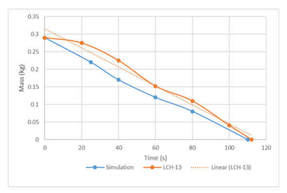 | Figure 10. Mass of liquid cryogen remaining with time for LCH13 |
Figure 10 and 11 shows that the simulation results agree rationally with the experimental data; and that the numerical experiments have predicted vaporization time about 9.4% lower than the experimental value in case of LCH-13. This suggests that the model suggested slightly higher vaporisation rates of LNG compared to the experimental values. This could be attributed to the influence of turbulence, consequently leading to higher heat transfer coefficients than the observed experimental values. The meager deviation is probably because in the experimental procedure of [16], the LNG was delivered onto water surface by pouring it along the sides, thereby successfully dampening the influence of turbulence effects on the vaporization rate of the LNG to a certain degree.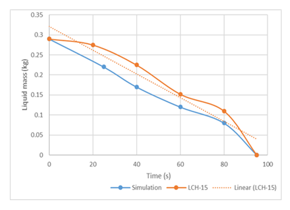 | Figure 11. Mass of liquid cryogen remaining with time for LCH15 |
The most probable source of error responsible for the observed disagreement between the model prediction of this work and the experiment of Boe [16] could be attributed to heat loss due to poor thermal insulation of their experimental set-up. As can be seen from Figure 10 and 11, the model under predicts the experimental boil-offs. This also might be due to the extra heat supplied to the cryogen through the walls of the boiling cell which led to higher boil-off of the cryogen than the predicted values. This is even evident as the observed mismatch between the model and Boe’s [16] experiment was higher for LCH-I3 which the initial temperature of water was 20°C.
4.3.3. Comparison with Zubairu & Velissa’s Numerical Experiment
Zubairu & Velissa [13], carried out a numerical experiment of LNG spill on water by developing a model that evaluates the water surface temperature and examine its influence on the rate of vaporization of LNG. Similar to Valencia-Chavez’s [2] experiment, Zubairu and Velissa [13] simulated LNG as pure liquid methane. Moreover, their simulation considered spill on both confined and unconfined water surfaces. The model in this work was simulated using their experimental conditions for unconfined spill while accounting for turbulence effects and the results were compared. The turbulence factor computed from Valencia-Chavez’s [2] experimental runs was used. As can be seen from Figure 12, that it took about 160 s for the 50,000 kg of spilled LNG to completely vaporize from the pool in Zubairu and Velissa [13] model. Using same experimental conditions, the model was simulated and it took the spilled cryogen about 80 s to completely vaporize. That amounts to about 50% decrease in the vaporization rate. Their model further indicates that overlooking the influence of turbulence effects grossly overestimates vaporization rate of LNG.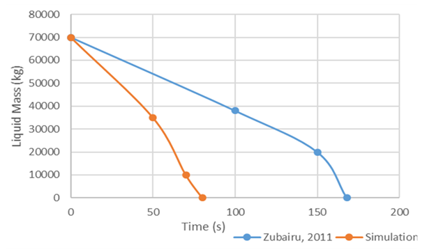 | Figure 12. Comparison of model simulation to Zubairu & Velissa’s [13] numerical experiment |
4.3.4. Comparison with Conrado and Vesovic Numerical Experiment
Conrado & Vesovic [10] studied the influence of chemical composition on vaporisation of LNG and LPG on unconfined water surfaces. Using their numerical experimental conditions, the model was run, and the sensitivity of LNG composition on the rate of vaporization of liquid spill was studied. In the idealized case, LNG was assumed to completely boil in the film boiling regime while maintaining constant heat transfer coefficient independent of changes in the composition of vapour film. Furthermore, they simulated the spills with and without the presence of wind action. In the simulation of this work using the conditions considered by [10], calm water surface (no wind effect) was considered as wind effects and wave actions were neglected. Figure 13 compares the simulation result of this work with that of [10]. We can see that the mass boil-off of LNG in our simulation is higher than that of [10]. Additionally, it could be seen that there was about 30 s difference in the vaporization time of the spilled LNG.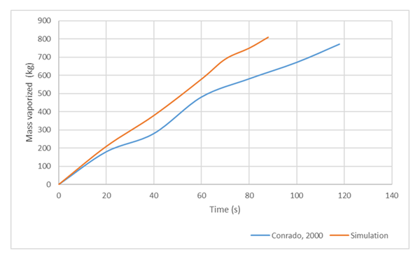 | Figure 13. Comparison of model simulation to Conrado & Vesovic [10] numerical experiment |
5. Conclusions
The influence of turbulence on fluid dynamics and heat transport due to LNG spill on water surface was successfully modelled and validated against previous works in the literature. The influence of water turbulence on other aspects of the boiling process was examined by comparing simulation results from this work with other experimental conditions obtained using theoretical heat transfer coefficients. The numerical simulation compared with experimental data from literature indicates an average of 10% deviation thereof, suggesting good fit of the model to experimental data.
References
| [1] | Basha, O., Liu, Y., Castier, M., Olewski, T., Vechot, L., and Mannan, S. (2013). Modelling of LNG Pool Spreading on Land with Included Vapour-Liquid Equilibrium and Different Boiling Regimes. Chemical Engineering Transactions, 31, 43-48. doi:10.3033/CET10331008. |
| [2] | Valencia-Chavez. (1979). The effect of composition on the boiling rates of Liquified NG for confined spills on water. International Journal of Heat and Mass Transfer, 428. |
| [3] | Zubairu, A. (2011). Modelling LNG Spills on Water: Heat Transfer Aspects. London: Imperial College. |
| [4] | Fay, J. A. (2003). Model of spills and fires from LNG and oil tankers. 96(April 2002), 171–188. |
| [5] | Betteridge, S., Technology, S., Thornton, C., Box, P. O., Hoyes, J. R., Gant, S. E., … Hill, H. (2011). Consequence modelling of large LNG pool fires on water Phoenix LNG Experiments at Sandia. 2009(159), 1–11. |
| [6] | Hightower, M., Gritzo, L., Luketa-hanlin, A., Covan, J., Tieszen, S., Irwin, M., … Ragland, D. (2004). Guidance on Risk Analysis and Safety Implications of a Large Liquefied Natural Gas ( LNG ) Spill Over Water. |
| [7] | Luketa-Hanlin, A. (2006). A review of large-scale LNG spills: Experiments and Modelling. Journal of Hazardous Materials, 119-140. |
| [8] | Hissong, D. W. (2006). Keys to modeling LNG spills on water. Journal of Hazardous Materials, 140(3), 465-477. doi: 10.1016/j.jhazmat.2006.10.040. |
| [9] | Vesovic, V. (2007). Influence of Ice formation on vaporization of LNG during spill on water surfaces. Journal of Hazardous Materials, 140(3), 518-526. |
| [10] | Conrado, C. and Vesovic, V. (2000, April 3). The Influence of Chemical Composition on Vaporization of LNG and LPG on Unconfined Water Surfaces. Chemical Engineering Science, 55, 4549-4562. |
| [11] | Opschoor, G. (1980). The Spreading and Evaporation of LNG and Burning LNG Spills on Water. Journal of Hazardous Materials, 3, 249-266. |
| [12] | Klimenko, V. (1981). Film Boiling on a Horizonatal Plate - New Correlation Int J. Heat Mas. International Journal of Heat and Mass Transfer, 24, 69–79. |
| [13] | Zubairu, A. and Velissa, V. (2011). Quantifying hazards associated with LNG release: vaporization rates. 20th World Petroleum Congress. Doha. |
| [14] | Hoult, D. (1972). Oil spreading on the sea. Annual Review of Fluid Mechanics, 341(1). Retrieved from http://www.annualreviews.org/doi/pdf/10.1146/annurev.f. |
| [15] | Guerra, A. (2001). Modelling the vaporization rate of LNG. MSc. thesis. London: Imperial College. |
| [16] | Boe, R. (1998). Pool boiling of hydrocarbon mixtures on water. International Journal of Heat and Mass Transfer, 1003–1011. |

 Abstract
 Reference
 Full-Text PDF
 Full-text HTML