Papiya Debnath1, Sanjay Sen2
1Department of Basic Science and Humanities, Techno India College of Technology, Kolkata, India
2Department of Applied Mathematics, University of Calcutta, Calcutta, India
Correspondence to: Papiya Debnath, Department of Basic Science and Humanities, Techno India College of Technology, Kolkata, India.
| Email: |  |
Copyright © 2014 Scientific & Academic Publishing. All Rights Reserved.
Abstract
A long strike-slip fault is taken to be situated in a viscoelastic half space. The material is taken to be of linear viscoelastic type combining both the properties of Maxwell and Kelvin-Voigt type materials. Tectonic forces due to mantle convection and other related tectonic processes are taken to be acting on the system, the magnitude of which is assumed to be slowly increasing with time. Expressions for displacement, stresses and strain are obtained both in the absence of fault movement and also after the creeping movement across the fault. Relevant mathematical techniques involving integral transform, Green's function, correspondence principle with suitable numerical methods have been used for solving the associated boundary value problem.
Keywords:
Correspondence principle, Creeping movement, Linear viscoelastic material, Mantle convection, Stress accumulation, Strike-slip fault
Cite this paper: Papiya Debnath, Sanjay Sen, Creeping Movement across a Long Strike-Slip Fault in a Half Space of Linear Viscoelastic Material Representing the Lithosphere-Asthenosphere System, Frontiers in Science, Vol. 4 No. 2, 2014, pp. 21-28. doi: 10.5923/j.fs.20140402.01.
1. Introduction
In the present paper we have considered a long vertical strike-slip fault situated in a viscoelastic half space. Most of the earlier works dealt with elastic/viscoelastic half space of Maxwell type or elastic/viscoelastic layered medium. But the properties of the material in the lithosphere-asthenosphere system suggest that other types of viscoelastic material may also be relevant. With this in view, we introduce linear viscoelastic material to represent the lithosphere- asthenosphere system having the properties of both Maxwell and Kelvin-Voigt type. Further the tectonic forces which cause movement across the earthquake faults in the region may not remain constant for the entire aseismic period in between two major seismic events, but is likely to be slowly increasing in nature. Consequently the tectonic force  is taken to be slowly increasing linearly with time. The resulting boundary value problems are solved by using integral transform, Modified Green's function technique and Correspondence principle.
2. Formulation
We consider a long strike-slip fault F of width D situated in a viscoelastic half space of linear viscoelastic material.We introduce a rectangular Cartesian coordinate system  such that the free surface is the plane
  and the fault is in the plane
  .
.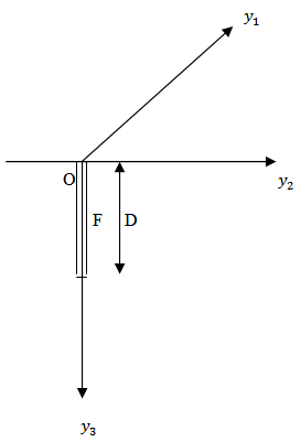 | Figure 1. The section of the model by the plane y1 = 0 |
We assume that for the long fault whose length is much greater than its width D, the displacement, stresses and strains are independent of  and depended on
  and t. With this assumption, the displacement, stress and strain components are separated out into two distinct groups: one group containing u,
  associated with strike-slip movement, while the other group containing
  associated with a possible dip-slip movement. We consider here the components of displacement, stress and strain u,
  associated with strike-slip movement across the fault. Similar model for a dip-slip fault was considered in [1].
2.1. Constitutive Equations (Stress-Strain Relations)
For the linear viscoelastic type medium combining both the properties of Maxwell and Kelvin-Voigt type materials, the constitutive equations have been taken as: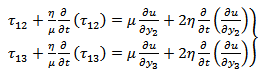 | (1) |
where  is the effective viscosity and
  is the effective rigidity of the material.
2.2. Stress Equation of Motion
We consider the aseismic state of the model when the medium is in a quasi-static state, and choose our time origin t=0 suitably. For slow, aseismic deformation, the stresses satisfy the following equation of motion as: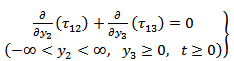 | (2) |
neglecting the inertial term.
2.3. Boundary Conditions
The boundary conditions are: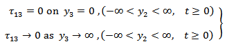 | (3) |
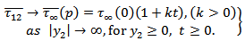
We assume  , the stress maintained by different tectonic phenomena including mantle convection, a slowly linearly increasing function with time, as
 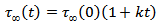 , where
  , is a small quantity. It is the main driving force for any possible strike-slip motion across F.
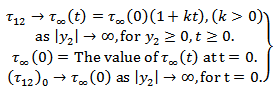 | (4) |
2.4. Initial Conditions
Let  and
and  are the values of u,
  ,
,  respectively at time t=0. They are functions of
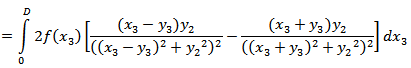
  and satisfy the relations (1) to (4).Now differentiating partially equation (1) with respect to
  and with respect to
  and adding them using equation (2) we get,
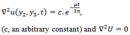 | (5) |
3. Displacements, Stresses and Strains in the Absence of Any Fault Movement
The boundary value problem given by (1)-(5) can be solved by taking Laplace transform with respect to time t of all constitutive equations and boundary conditions. Finally, on taking inverse Laplace transform we get the solutions for displacement, strains and stresses as: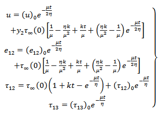 | (6) |
From the above result we find that, the initial field for displacement, stresses and strain gradually dies out. The relevant stress component  is found to increase with time t and tends to
  as
as . However the rheological behaviors of the material near the fault F are assumed to be capable of withstanding stress of magnitude
  , called critical value of the stress where
  is less than
  . We assume that when the accumulated stress
  near the fault exceeds this critical level after a time, T, a creeping movement across F sets in, and thereby the accumulated stress releases to a value less than
  .If we assume
  ,
,  ,
,  and
and  , it is found that
  reaches the value
  in about 96 years. In our subsequent discussions we shall take T to be 96 years.The relevant boundary value problem after commencement of the creeping movement across F,
  has been described in Appendix-7.2.
4. Displacements, Stresses and Strains after the Commencement of the Fault Creep
We assume that after a time T, the stress component  which is the main driving force for the strike-slip motion of the fault, exceeds the critical value
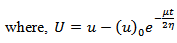
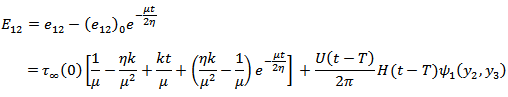
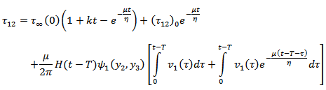
  and the fault starts creeping characterized by a dislocation across the fault as discussed in Appendix-7.2.We solved the resulting boundary value problem by modified Green's function method following [2], [3] and correspondence principle (as shown in Appendix) and get the solution for displacement, strain and stresses as:
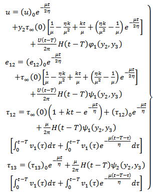 | (7) |
where  ,
,  and
and  are given in the Appendix.It has been observed, as in [4] that the strains and the stresses will be bounded everywhere in the model including the lower edge of the fault, the depth dependence of the creep function
  should satisfy the certain sufficient conditions:(I)
  ,
,  are continuous in
  ,(II) Either (a)
  is continuous in
  or (b)
  is continuous in
  except for a finite number of points of finite discontinuity in
  ,or (c)
  is continuous in
  , except possibly for a finite number of points of finite discontinuity and for the ends points of (0,D), there exist real constants m<1 and n<1 such that
  or to a finite limit as
  and
and 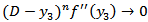 or to a finite limit as
  and(III)
 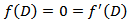 ,
,  ,These are sufficient conditions which ensure finite displacements, stresses and strains for all finite
  including the points at the lower edge of the fault.We can evaluate the integrals in
 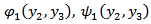 and
and  in the above equations in closed form, if
  is any polynomial satisfying (I), (II) and (III). One such function is
5. Numerical Computations
We consider  to be
to be  which satisfies all the conditions for bounded strain and stresses stated above.Following [5], [6] and the recent studies on rheological behaviour of crust and upper mantle by [7], [8], the values to the model parameters are taken as:
 D = Depth of the fault = 10 km., noting that the depth of the major earthquake faults are in between 10-15 km.
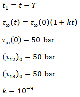
6. Discussion of the Results
We compute the following quantities: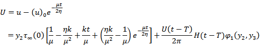
 where the expression for u,
  are given in expression (7).
6.1. Displacement against Year
Figure 2 shows surface displacement against time due to the effect of  and the creeping movement across the fault with
  .It has been observed that in the absence of the fault movement the displacement increases almost linearly with time at a slightly increasing rate. After the onset of the creeping movement across the fault at t = 96 years the displacement increases almost linearly but at much higher rate. This sudden increase may be attributed to the creeping movement across the fault.
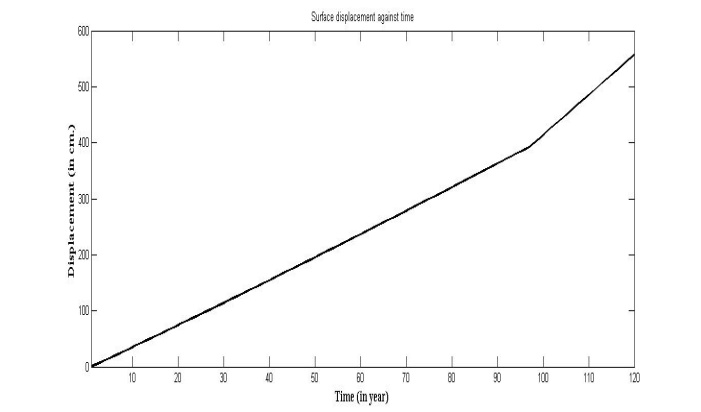 | Figure 2. Surface displacement against time (y2 = 10 km) |
6.2. Displacement against y2
Figure 3 shows surface displacement against  , the distance from the fault, just before and after commencement of the fault movement.
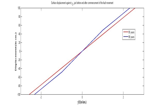 | Figure 3. Surface displacement against y2, just before and after commencement of the fault movement |
It is observed from the figure that the displacement increases at a constant rate as expected for t=95 years (just before the commencement of the fault movement). The curve in the red colour shows the displacement against  for t=98 years just after the beginning of the fault movement. Comparing these two curves it is found that the magnitude of the displacement is always greater in the later case. The displacement increases but with a gradually decreasing rate.
6.3. Strain against Year
Figure 4 shows Surface share strain before the commencement of the fault movement.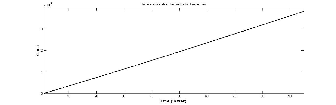 | Figure 4. Surface share strain before the fault movement |
We can deduce from the figure that the share strain increases slowly with time under the action of  but its magnitude is found to be of the order of
  which is in conformity with the observational facts.
6.4. Stress near the Midpoint on the Fault (y2=0.5 km. and y3= 5.0 km.) Against Time for Different Creep Velocities
Figure 5 shows that, in the absence of any fault movement across F, the share stress  increases gradually with time but at a decreasing rate. After the commencement of the fault movement the stress accumulation pattern near the fault undergoes significant changes depending upon the creep velocity (v). For v=10 cm./year the rate of accumulation decreases significantly. For v=20 cm./year the accumulation rate is marginally above zero. For higher values of v, the stress gets released instead of accumulation. For example for v=50 cm./year the accumulated stress has been completely released within 60 years after the commencement of the fault movement.
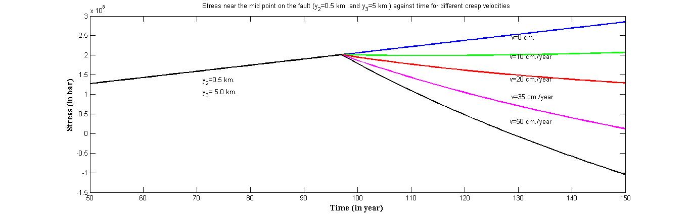 | Figure 5. Stress near the mid point on the fault (y2 =0.5 km. and y3 = 5.0 km.) against time for different creep velocities |
6.5. Stress against Depth
In Figure 6 the stress  along the fault due to the movement across F where,
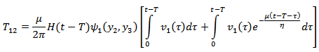 The magnitude of
  has been computed very close to the fault line with y2 =0.5 km. and y3 varies from 0 to 50 km. The figure shows that initially the stress is negative and its magnitude increases up to a depth of 2 km. from the upper edge of the fault. Thereafter its magnitude decreases up to the lower edge of the fault, where its attends its maximum positive value at y3 =10 km. As we move downwards the accumulated stress gradually dies out and tends to zero.
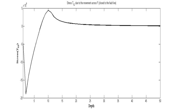 | Figure 6. Stress T12 due to the movement across the F (closed to the fault line) |
6.6. Stress against Depth and y2
Figure 7 shows Identification of the region of stress accumulation and stress reduction due to the creeping movement across F.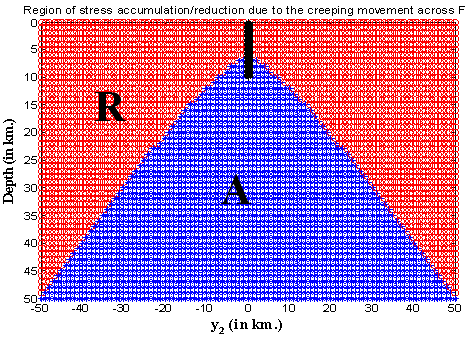 | Figure 7. Region of stress accumulation/reduction due to the creeping movement across F |
We computed  for a set of values of
  from -50 km. to 50 km. and for a set of values of
  ranging from 0 km. to 50 km. It is found that, there is a clear demarcation of the zones where stress is increased due to the fault movement marked by (A: Blue in the graph) and a stress reduction zone (R: Red in the graph). From this figure we may conclude that if there be a second fault situated in the region of stress accumulation (marked A) then the rate of accumulation of stress near it will be increased due to the movement across the fault F. As a result, the time of a possible movement across the second fault will be advanced. On the other hand if the second fault be situated in the region of stress reduction (marked by R), the rate of stress accumulation near the second fault will be reduced due to the fault movement across F and as a result any possible movement across the second fault will be delayed due to the movement across F. This gives us some ideas about the interactions among neighboring faults in a seismic fault system. The interacting effects depend on the relative positions of the fault.
ACKNOWLEDGEMENTS
One of the authors (Papiya Debnath) thanks the Principal and Head of the Department of Basic Science and Humanities, Techno India College of Technology, a unit of Techno India Group (INDIA), for allowing me to pursue the research, and also thanks the Geological Survey of India; Department of Applied Mathematics, University of Calcutta for providing the library facilities.
Appendix
A1. Displacements, Stresses, and Strains before the Commencement of the Fault Creep
The method of solutionWe take Laplace Transform of all constitutive equations and boundary conditions | (8) |
where 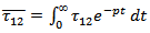 , p being the Laplace transform variable.Also the stress equation of motion in Laplace transform domain as:
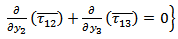 | (9) |
and the boundary conditions are (after transformation)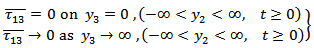 | (10) |
 | (11) |
Using (8) and other similar equation assuming the initial fields to be zero, we get from (9) | (12) |
Thus we are to solve the boundary value problem (12) with the boundary conditions (10) and (11)Let, 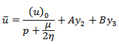 be the solution of (12), where
 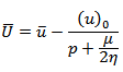 Using the boundary conditions (10) and (11) and the initial conditions we get,
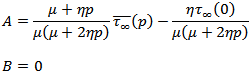 On taking inverse Laplace transform, we get
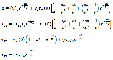
A2. Displacements, Stresses and Strains after the Commencement of the Fault Creep
The method of solutionWe assume that after a time T the stress component  , which is the main driving force for the strike-slip motion of the fault, exceeds the critical value
  , the fault F starts creeping then (8) to (11) are satisfied with the following conditions of creep across F:
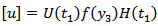 | (13) |
where  is the discontinuity in u across F, and
  is Heaviside unit step function.That is
 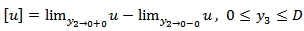 | (14) |
The creep velocity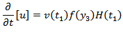 where
where 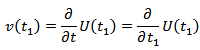 and
and  vanish for
  .Taking Laplace transform in (13) with respect to
  , we get
 | (15) |
The fault creep commence across F after time T, we take
 We try to find the solution as:
 | (16) |
where  are continuous everywhere in the model satisfying equations (1) to (5). The solution for
  are similar to equation (6).For the second part
  and
and  boundary value problem can be stated as:
 | (17) |
where  is the Laplace transformation of
  with respect to t, give
 The modified boundary condition:
 | (18) |
and the other boundary conditions are same as (10) and (11).Now we solve the boundary value problem by using a modified Green's function technique developed by [1], [2] and the Correspondence Principle.Let,  is any point in the medium and
  is any point on the fault, then we have
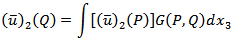 where the integration is taken over the fault F. Therefore,
 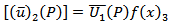 where G is the Green's function satisfying the above boundary value problem and
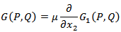 where
where
 Now,
Now,  where
where  We assume that
  is continuous everywhere on the fault
  .Now, taking inverse Laplace transformation
 where
where  is Heaviside unit step function, and
 where
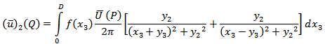
where  is the depth-dependence of the creeping function across F.We also have,
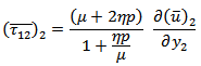 and similar other equations.Now, taking inverse Laplace transformation we get
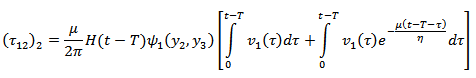 where
where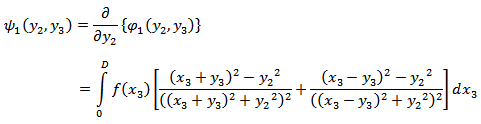 Similarly,
 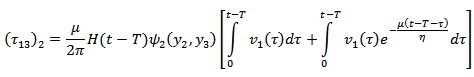 where
where 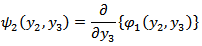
References
| [1] | Sen, S., Debnath, S.K. “ Stress and strain accumulation due to a long dip-slip fault movement in an elastic layer over a viscoelastic half space model of the lithosphere- asthenosphere system”, International Journal of Geosciences, 4, pp. 549-557, 2013. |
| [2] | Maruyama, T. “On two dimensional dislocation in an infinite and semi-infinite medium”, Bull. earthquake res. inst., tokyo univ., 44, part 3, pp. 811-871, 1966. |
| [3] | Rybicki, K., “Static deformation of a multilayered half-space by a very long strike-slip fault”, Pure and Applied Geophysics, 110, p-1955-1966, 1973. |
| [4] | Mukhopadhyay, A. et.al. “On stress accumulation near a continuously slipping fault in a two layer model of lithosphere”, Bull. Soc. Earthq. Tech., vol.4, pp. 29-38. (with S. Sen and B. P. Pal), 1980b.17. |
| [5] | Catlhes III, L.M., “The viscoelasticity of the Earths mantle”, Princeton University Press, Princeton, N.J, 1975.15. |
| [6] | Aki, K., Richards, P.G., “Quantitive Seismology”, University Science Books, Second Ed., 1980. |
| [7] | Chift, P., Lin, J., Barcktiausen, U., Marine and Petroleum Geology: 19, 951-970, 2002. |
| [8] | Karato. S.I. (July, 2010): “Rheology of the Earth's mantle,’’ A historical review Gondwana Research, vol-18, issue-1, pp-17-45. |
 Abstract
 Reference
 Full-Text PDF
 Full-text HTML