1. Introduction

Wikipedia defines Global Warming as the increase in the average temperature of the Earth's near-surface air and oceans since the mid-20th century and its projectedstatistical model to predict CO₂ in the atmosphere taking into consideration eight attributable variables to the subject matter. The eight attributable variables are namely, CO₂ emission (E), deforestation and destruction of biomass and soil carbon (D), terrestrial plant respiration (R), respiration from soils and decomposers (S), the flux from oceans to atmosphere (O), terrestrial photosynthesis (P), the flux from atmosphere to oceans (I ), the burial of organic carbon and limestone carbon in sediments and soils (B).

We need to mention here that some of the attributable variables are the function of several other variables within themselves. For example, CO₂ emission, E, is a function of six attributable variables namely, Gas fuels (Ga), Solid fuels (So), Liquid fuels (Li), Gas Flares (Fl), Cement (Ce) and Bunker (Bu). Gas fuels include gas consisting primarily of methane. They includenatural gas and other gases that can provide energy through combustion. Solid fuels refer to various types of solid material that are used as fuel to produce energy and provide heating, usually released through combustion. Solid fuels include wood, charcoal, coal and others. Liquid fuels are those combustible or energy-generating molecules that can be harnessed to create mechanical energy, such as the gasoline we normally use. Gas flares is the vertical stack on oil wells or natural gas well completion activities. Cement refers to theCO₂ generated through the production of cement. Bunker fuel is a type of crude oil also named heavy oil or furnace oil. It belongs to the heavy fractions or hard to distill fractions when crude oil is refined and often used for ships.

The proposed model that we are developing takes into consideration individual contributions and interactions along with higher order contributions if applicable. In developing the statistical model, the response variable is the CO₂ in the atmosphere and is given in unit parts per million (PPM). In the present analysis, we used real yearly data that has been collected from 1959 to 2004 for the continental United States. The air samples were collected at Mauna Loa Observatory, Hawaii. The CO₂ emission data was obtained from Carbon Dioxide Information Analysis Center (CDIAC). The CDIAC is the primary climate-change data and information analysis center in the U.S. Department of Energy (DOE), located at Oak Ridge National Laboratory (ORNL) and includes the World Data Center for Atmospheric Trace Gases. All emission estimates are expressed in thousand metric tons of carbon (MT). Carbon emissions are calculated by the fuels consumed times the heat coefficient times the carbon coefficient times the combustion efficiency. The product of the fuels consumed times heat coefficient is in the unit of trillion Btu. The carbon coefficients are given by the Environmental Protection Agency (EPA) reports[1].It is the amount of carbon that is emitted per unit of heat realized from combustion. Petroleum data was obtained from DOE report, and are published in the Monthly Energy Review [2], [3], [4].

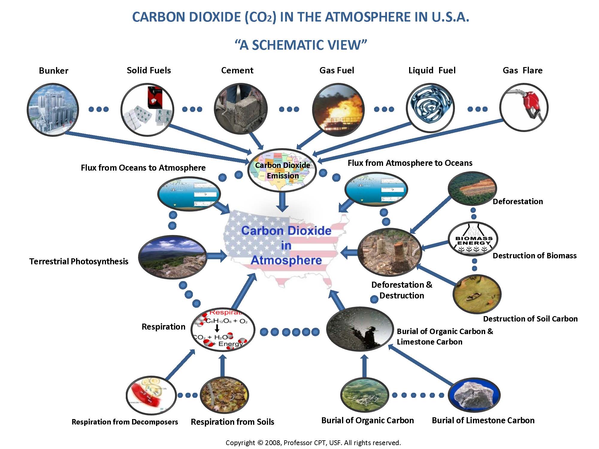Figure 1. Carbon Dioxide in the Atmosphere in U.S.A

A schematic diagram that shows the relationship between the attributable variables and carbon dioxide in the atmosphere is given by Figure 1.

The proposed statistical model is useful in predicting the CO₂ in the atmosphere given the information of attributable variables. It has been statistically evaluated using R square, R square adjusted, PRESS statistic and residual analysis. Finally, its usefulness has been illustrated by utilizing different combinations of various attributable variables. To our knowledge, no such model has been developed under the proposed analytical structure.

In addition, we rank the attributable variables according to their CO₂ contributions in the atmosphere.

2. Historical Review

Hansen (1984) discuss the climate processes and climate sensitivity [5]. Lashof (1989) analyze the feedback processes that may influence future concentrations of atmospheric trace gases and climate change [6]. Thomas J. Goreau (1990) stated the eight attributable variables for CO₂ in the atmosphere [7]. Retallack (2002) generally talk about the understanding climate change. Shih and Tsokos (2008) proposed a forecasting model for temperature and carbon dioxide for the United States and they suggest a weighted moving average procedure for forecasting [8], [9], [10]. Hachett and Tsokos (2009) discovered a new method for obtaining a more effective estimate of atmospheric temperature in the united states [11].Tsokos and Xu (2009) have proposed differential equations for individual attributable variables for CO₂ emission and cumulatively [12]. The parametric analysis for CO₂ has been studied extensively by Wooten and Tsokos (2010) [13]. They have found that the CO₂ data follows the three parameter Weibull probability distribution contrary to the fact that some scientists believed that CO₂ in the atmosphere follows Gaussian probability distribution. Xu and Tsokos (2011) have proposed an overall model to modeling the CO2 in the atmosphere and all possible attributable variables [14]. Several other recent researches can be found in [15], [16] and [17]. In this study we will follow up the research in [14] to construct an improved overall model for those significant attributable variables and the cumulatively CO₂ in the atmosphere. We will use the most updated data to construct this model and we will show the improvement in the result.

The illustration of Carbon dioxide circulation process in the atmosphere that was developed by scientists at the Oak Ridge National laboratory is given by Figure 2, below. (from ICPP’s report)

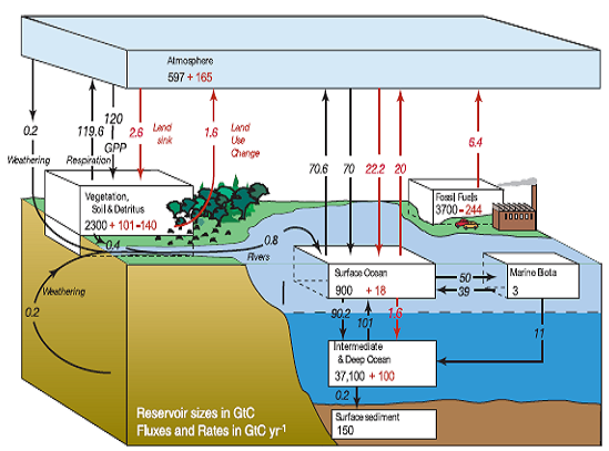Figure 2. CO2 Circulations in Atmosphere

3. Development of Nonlinear Statistical Model

We proceed to develop a statistical model taking into consideration the eight attributable variables as presented previously. The form of the statistical model is given by CO₂ in the atmosphere as a function of temperature. Thus, the statistical form of the model with all possible interactions will be

(3.1)

Here the and are the coefficients and A are the first order term of the attributable variables and B are the possible interactions and higher order terms. The object is to develop the most representative estimate of the above model based on available data. In the present study we will focus on using atmospheric CO₂ as response and only six attributable variables as our independent variables. For the overall model that considers all possible attributable variables, please check the Xu and Tsokos paper 2010.

The data comes from Oak Ridge National Lab: Division of U.S. Department of Energy. The plot of CO₂ in the atmosphere is shown in Figure 3, below. The air samples collected at Mauna Loa Observatory, Hawaii and the data unit is in ppmv.

One of the underlying assumptions to construct the above model 3.1 is that the response variable should follow Gaussian distribution. We know the CO₂ in the atmosphere are not follow Gaussian distribution which can be clearly seen from the QQ plot shown by Figure 4, below.

We will utilize Box-Cox transformation to the CO₂atmosphere data to filter the data to be normally distributed. After we proceed with the Box-Cox transformation, the results are shown in Table 1.

Table1. Box-Cox Transformation for Normality Est. Power Std. Err Wald (Power=0) Wald (Power=1) -2.3763 .9609 -2.4729 -3.5136

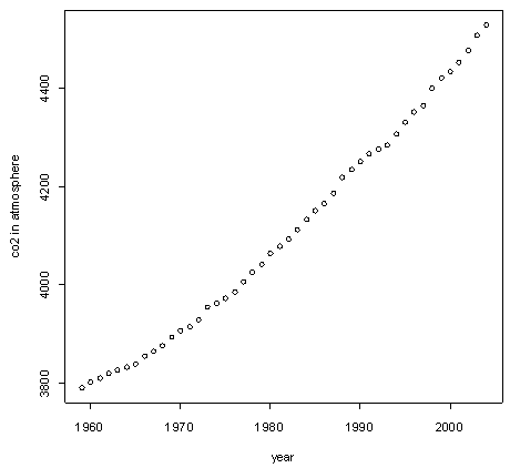Figure 3. Yearly CO2 in Atmosphere Data at Mauna Loa

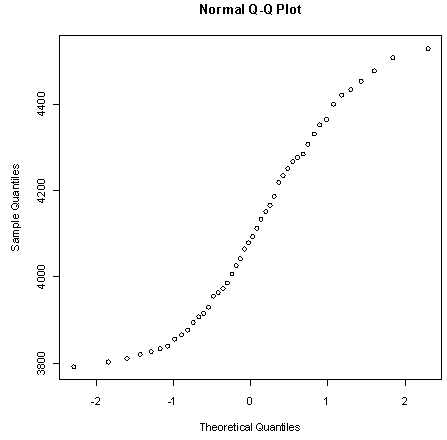Figure 4. QQ Plot for Testing Normality

After the Box-Cox filter, we retest the data and it shows our data will follow normal distribution; thus, we proceed to estimate the coefficients of the contributable variables for the transformed CO₂atmosphere data in the equation 3.1.

We can proceed to estimate the approximate coefficients of the contributable variables for transformed CO₂ in the atmosphere and obtain the coefficient of all possible interactions. At the same time, we candetermine the significant contributions of both attributable variables and interactions.

We begin with sixattributable variables as previously defined, such as Ga,So,Li,Fl,Ce, and Bu and fifteen 2nd order interactions between each pair. To develop the models, initially we start building our model with 21 total terms that include initial contribution of attributable variables and all possible interactions. We construct twenty-foursuch models.

During our statistical analysis in the estimation process, we found only oneout of six attributable variables significantly contribute and five interaction terms. Thus the result of estimation of equation 3.1 is given by equation 3.2 as follows

(3.2)

We will utilize the initial transformation that we used to transform the response data to get the result in equation 3.3 by taking the (-.4208)’s power on both sides of the equation 3.2.

(3.3)

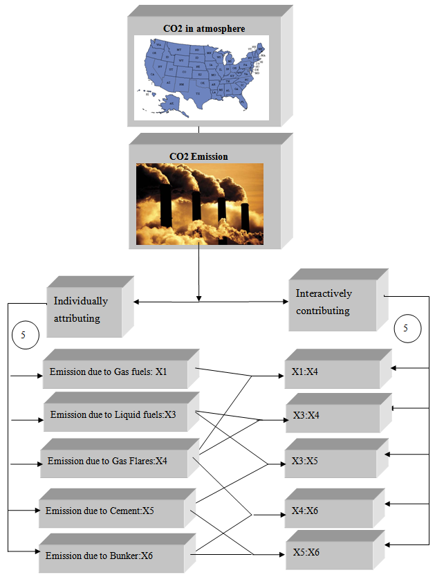Figure 5. CO2 in the AtmosphereAttributable Variable Diagram

This proposed nonlinear statistical model identifies the following attributable variables. We can find Ca, Li, FL, Ce and Bu significantly contribute to the CO₂. Furthermore, we have identified the following interactions that have been show statistically contribute to CO₂ namely Ga*FL, Li*FL, Li*Ce, FL*Bu and Ce*Bu. We summarized our model in the Figure 5.

The proposed underlying statistical model is high in quality.It has been evidenced by high value of both R square and R square adjusted which are the key criteria to evaluatethe model fitting. The regression sum of squares (SSR), also called the explained sum of squares, is the variation that is explained by the regression model. The sum of squared errors (SSE), also called the residual sum of squares, is the variation that is left unexplained. The total sum of squares (SST) is proportional to the sample variance and equals the sum of SSR and SSE. The coefficient of determinationis defined as the proportion of the total response variation that is explained by the model. It provides an overall measure of how well the model fits. R-square is SSR/SST.R-square adjusted will adjust for degree of freedom of the model and it works better when we have many parameters. R-square adjusted is

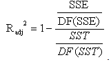The prediction of residual error sum of squares (PRESS) statistics will evaluate how good the estimation will be if each time we remove one data point and PRESS is defined

For our final model the R squared is 0.9963 and R squared adjusted is 0.9953. Both R squared and R squared adjusted are very high (more than 90%) and these two are very close to each other. This shows our model’s R squared increase in not due to the increase of the parameters estimates but the good quality of the proposed model to predict CO₂ in the atmosphere given values of the identified attributable variables[2]. Secondly, the PRESS statistics results support the fact that the proposed model is of high quality. We will list the best three models’ PRESS statistic out of total 28 and the result is in Table 2, below. From the table it is clear that the best model is number 28, which is our final model.

Table 2. PRESS Statistics for Best Three Models Model number PRESS value Rank of the model 24 3.414703e-20 1 23 3.523170e-20 2 19 8.1202e-20 3

Furthermore, R square and R square adjusted are calculated for those 28 models which are of interest but the proposed model gives the best possible estimates of the CO₂ in the atmosphere. We just present the best possible model’s statistical evaluation criteria in Table 3.

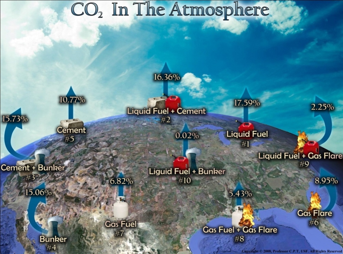Figure 6. CO2 in the AtmosphereAttributable VariableContribution Diagram

Table 3. Statistical Evaluation Criteria R square R square adjusted PRESS 0.9963 0.9953 3.414703e-20

The following Table 4 ranks the attributable variables with respect to their contribution to CO₂ in the atmosphere. As we expected, Li ranks number one which is one of the attributable variables from the emissions from fossil fuels. The individual contributions with interactions are shown in Figure 6, below. We ranked those terms by their percentage of contribution to CO₂ in the atmosphere.

Table 4. Rank of Variable According to Contributions Rank Variables 1 Liquid 2 Liquid: Cement 3 Cement: Bunker 4 Bunker 5 Cement 6 Gas Flares 7 Gas Fuels 8 Gas Fuels: Gas Flares 9 Liquid :Gas Flares 10 Gas Flares: Bunker

4. Validation of the Proposed Model

We will utilize two methods to do the model validation. The first method is to use the proposed model to calculate the predicted value for each individual data and then calculate the residuals. The residual is defined as the original value minus the predicted value. Table 5 shows the last ten residuals out of the total one hundred fifty-five residuals.

The mean of the residuals is -.0286, variance of the residuals is 1.588, standard deviation is 1.26 and standard error of the residuals is .1012.

Table 5. Residual Analysis No Residual Values 37 -1.142226e-12 38 -4.122377e-12 39 1.764721e-11 40 4.939785e-12 41 -3.126147e-11 42 2.243955e-11 43 3.234128e-11 44 1.167639e-11 45 -2.728478e-11 46 -1.357971e-11

Table 6. Residual Analysis for Transformed Data Mean of Residual 3.645909e-28 Standard Deviation of Residual (SD) 2.020493e-11 Standard Error of Residual (SE) 5.832662e-12

The second method we will utilize is the cross validation. The basic idea is we will save some part of the data as validation part. We construct our model using only the data left and the constructed model will be same structure as our proposed model with only coefficients being different. We will test the quality of model using three settings.

We will first randomly divide the data into two data sets of same size. Then we will use one to construct the model and then use this model to predict the value using other data set’s attributable variables. Then we will switch the two data sets and repeat the procedure. The mean of all residuals is 1.052026e-21.

Second we will divide the data set into six small data sets and use five of them to construct the model and validate the model using the sixth one. Then we will repeat the same procedure for each of the six small data sets. The mean of all residuals is 8.378600e-22.

Table 7. Residual Analysis for Cross Validation No Residual Values 37 3.445021e-24 38 3.113447e-23 39 7.893401e-22 40 3.354917e-23 41 2.003004e-21 42 1.836528e-21 43 1.760729e-21 44 1.938752e-22 45 1.886689e-21 46 5.623131e-22

Thirdly, we will divide the data set into 46 data sets and use all 45 sets to construct the model and validate the model using the one left out. Then we repeat the procedure 46 times. Table 7 shows the last ten residuals out of the total 46 residuals.

The mean of the residuals is 7.423267e-22, variance of the residual is 7.007e-43, standard deviation is 8.371e-22 and standard error of the residuals is 8.370868e-22.

5. Usefulness of the Proposed Model

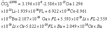
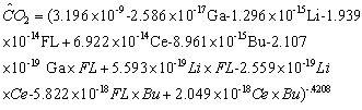
We can conclude from our extensive statistical analysis that there are only five significant attributable variables to the CO₂ in the atmosphere namely, Gas fuels, Gas flares, Bunker, Liquid and Cement. Furthermore, we also tested all possible 2^nd order interactions of allattributable variables and we found only five interactions that significantly contribute to CO₂ in the atmosphere, namely, Liquid with Cement, Cement with Bunker, GasFuels with Gas Flares, Liquid with Gas Flares and Gas Flares with Bunker. Thus, one may obtain a good estimate of the CO₂ in the atmosphere by knowing the measurement of Cement and those five interactions.

One can utilize the above model equation 3.2 to perform surface response analysis to identify the values of the contributable variables that will minimize the CO₂ in the atmosphere.

6. Conclusions & Discussion

In the present study, we have performed parametric analysis for CO₂ in the atmosphere. The initial measurement of CO₂ in the atmosphere was collected at Mauna Loa Observatory, Hawaii (C.D. Keeling, T.P. Whorf, 2005). Those data do not follow normal probability distribution. Thus, we transform the response of the data by using Box-Cox transformation that resulted in make the CO₂ being normal. The developed statistical was validated and is extremely accurate. Using this model we have identified the important and unique information that only five attributable variables, namely liquid, bunker, cement, gas flares, and gas fuels significantly contribute to the amount of CO₂ in the atmosphere along with five interactions, namely, liquid-cement, cement-bunker, gas fuels-gas flares, liquid-gas flares, and gas flares-bunker. Scientists working in the subject area list at least twenty attributable variables and no interactions that contribute to CO₂ in the atmosphere. The high accuracy of our predictive model is reflected by the values of R square and R square adjusted and the PRESS statistics. Furthermore, the statistical model was cross validated by hiding some actual CO₂ data and proceed to estimate the CO₂ from the model, the mean residuals of the cross validation is extremely small, that further reflects the accuracy of our results. We proceeded to use the statistical model to rank the attributable variable and interactions with respect to the percent amount of CO₂ they contribute in the atmosphere. Liquid fuels is number one with the interactions of gas flares and bunker contribute the minimum (number 10) significant amount of CO₂ in the atmosphere.

The developed statistical model can be used;

I. To estimate the CO₂ in the atmosphere.

II. Can be used for research funding allocations based on the ranking of the attributable variables.

III. Use the model and its findings to establish environmental policies to address the issues of CO₂ in the atmosphere.

IV. Develop economic models based on the present findings to assist in implementing the legal policies.

V. Use the developed statistical model to identify violation of the established legal policies.

ACKNOWLEDGEMENTS

The authors wish to acknowledge the assistance and suggestions of T.J. Blasing from Oak Ridge National Laboratory during the progress of the present study.