Shahriar Shirvani Moghaddam, Somaye jalaei
Digital Communications Signal Processing (DCSP) Research Lab., Faculty of Electrical and Computer Engineering, Shahid Rajaee Teacher Training University (SRTTU), 16788-15811, Lavizan, Tehran, Iran
Correspondence to: Shahriar Shirvani Moghaddam, Digital Communications Signal Processing (DCSP) Research Lab., Faculty of Electrical and Computer Engineering, Shahid Rajaee Teacher Training University (SRTTU), 16788-15811, Lavizan, Tehran, Iran.
| Email: |  |
Copyright © 2012 Scientific & Academic Publishing. All Rights Reserved.
Abstract
Determining the number of sources from observed data, is a fundamental problem in array signal processing. In this paper, first we focus on two popular estimators based on information theoretic criteria, AIC and MDL. Then another algorithm based on eigenvalue grads, namely EGM is presented. The computer simulation results prove the effective performance of the EGM for non-coherent signals but in the small differences between the incident angles of non-coherent sources, MDL and AIC have a much better detection performance than EGM. These methods can detect only non-coherent signals, and the performance of them will be sharply declined even signals are coherent and/or correlated. So, first forward/backward spatial smoothing (FBSS) method is used as a pre-processing step to solve the coherency/correlation, and then MDL, AIC and EGM algorithms are run to estimate the number of signals. Numerical results show that FBSS-based EGM offers higher detection probability rather than FBSS-based MDL and AIC in the case of coherent sources as well as correlated ones. Also, the higher detection probability can be achieved for correlated case compared to coherent one.
Keywords:
Information Theoretic Criteria, AIC, MDL, EGM, Coherent Signals, Correlated Signals, Spatial Smoothing, FBSS
Cite this paper:
Shahriar Shirvani Moghaddam, Somaye jalaei, "Determining the Number of Coherent/Correlated Sources Using FBSS-based Methods", Frontiers in Science, Vol. 2 No. 6, 2012, pp. 203-208. doi: 10.5923/j.fs.20120206.12.
1. Introduction
Wireless direction finding is the procedure for determining signal sources by observing signal direction of arrivals (DOAs). Its history came back to the beginning of wireless communications. This technology is used in many fields such as radar, sonar, mobile communications, astronomy, seismology and etc. So, DOA estimation using sensor arrays and direction finding, are important subjects in signal processing[1]. Most of the DOA estimation algorithms, assume that the number of sources is known a priori and may give misleading results if the wrong number of sources is used. So, determining the number of signals is an important problem in field of array signal processing[2]. In order to determine the number of sources to satisfy the requirement of DOA estimator, many parametric and nonparametric detection methods have been proposed[3]. A number of related methods have been widely studied in[4]. One of the most widely-used approaches is that of information theoretic criteria, which introduced by Wax and Kailath for the first time. They proposed an approach to this problem, based on the Akaike’s information criterion (AIC) and minimum description length (MDL). According to these two algorithms, the number of signal sources is determined as the value for which the AIC or MDL criterion is minimized[5].However, despite these methods are efficient in detection point of view, they involve the estimation of a covariance matrix and its eigenvalue decomposition which introduce generally high complexity. In order to reduce the computational complexity and attain accurate detection performance, a low-complexity MDL method is developed in[6]. This method employs the training data of the desired signal, to quickly partition the array data into two orthogonal components in signal and noise subspaces. To enhance the probability of detection, an accurate minimum description length (MDL) method was devised in[7]. Since the training sequence of the desired signal is used to calculate the minimum mean square error (MMSE), the performance of proposed method is significantly superior to the traditional MDL method at low SNRs and small number of snapshots. Luo Jing Qing[8] proposed a set of eigenvalue gradient methods (EGMs), which like AIC and MDL methods, it also determines the number of non-coherent sources according to the eigenvalues of auto-correlation matrix. Another algorithm that considers a bound or threshold for eigenvalues is investigated in[9]. This approach is a simple and efficient way to increase detection probability in the case of unequal power sources.Above discussed techniques assume that noise is spatially uncorrelated. In practice, signals experience colored noise which causes decreasing the performance of conventional methods, rapidly. To overcome this problem, a signal enumerator for spatially correlated noise has been proposed in[10]. They combine the combined information theoretic criteria and eigenvalue correction to estimate the number of coherent signals. Li Jing-hua and Li Rong[11] established a novel effective detection algorithm in spatial color noise by using the canonical correlation coefficients of the joint covariance matrix. Compared with the other algorithms, this algorithm has a better performance and lower complexityIn the real environment, the coherent source is common, and the above-mentioned methods are suitable for non-coherent signals, and their performance will be sharply declined even signals are coherent or correlated[12]. A partial solution to this problem, applicable to coherent or correlated sources, was proposed in[13]. The method uses the MDL principle and decomposes data into signal and noise components. The MDL descriptor is then computed for signal and noise components separately, and the results are added to obtain the total MDL cost. Another way is to use spatial smoothing (SS) method to solve the coherency/correlation, and then estimate the number of signals. Spatial smoothing scheme partitions the total array of sensors into sub-arrays and then generates the average of the sub-array output covariance matrices[14, 15]. The second method is more applicable because SS is a pre-processing required for both determining the number of sources and DOA estimation.The main purpose of this paper is to determine the number of sources in three types of sources, non-coherent, coherent, and correlated, based on MDL, AIC and EGM methods. First, conventional MDL, AIC and EGM algorithms are applied to detect the number of non-coherent sources. Then, by applying spatial smoothing as a pre-processing part, above mentioned algorithms are used for detecting the number of coherent/correlated sources.The paper is organized as follows. After the statement and formulation of the problem in Section 2, Section 3 presents the derivation of the three detection criteria for non-coherent sources (MDL, AIC and EGM). In addition, two experiments and associated simulation results are presented. Section 4 presents forward/backward spatial smoothing (FBSS) technique for determining the number of coherent/correlated sources. Moreover, it illustrates simulation results of two experiments, coherent and correlated sources. Finally, Section 5 concludes this research.
2. Signal Model
Consider  narrowband signals emitted from the far field impinging on array of
  sensors
  . The
. The  measurements of the output of the array corrupted by additive noise can be expressed as
  | (1) |
where  is the matrix of array manifold,
  is the vector of signal, and
  is the additive noise. The additive noise is assumed to be complex, ergodic Gaussian vector stochastic process, independent of the signals, with zero mean and covariance matrix given by
  [16]. The covariance matrix for array is
  | (2) |
where  is the correlation matrix of signals. In fact, considering ergodic processes, correlation matrix is acquired from limited data, that is
  | (3) |
where  is the number of snapshots. To solve the problem, determining the number of sources from
  we consider the following assumptions[13].1. The array manifold, defined as the set of steering vectors,
  is known.2. Any subset of
  steering vectors from the array manifold is linearly independent.3. The number of sensors is greater than the number of sources, namely,
3. Determining the Number of Non-coherent Sources
In this section, first, three well-known algorithms, MDL, AIC and EGM, are described for non-coherent signals. Consequently, related simulation results that show the performance of these algorithms are illustrated with more details.
3.1. Estimating the Number of Signals with Information Theoretic Criteria
The information theoretic criteria for model selection, introduced by Akaike Schwartz and Rissanen, address the following general problem: Given a set of  observation
  and a family of models, that is, a parameterized family of probability densities
  selects the model that best fits the data.Akaike’s proposal was to select the model which gives the minimum AIC, defined by
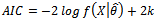 | (4) |
where  is the maximum likelihood estimate of the parameter vector
  , and
, and  is the number of free adjusted parameters in
  . Inspired by Akaike’s pioneering work, Schwartz and Rissanen approached the problem from quite different points of view. Rissanen’s approach is based on information theoretic arguments. Since each model can be used to encode the observed data, Rissanen proposed to select the model that yields the minimum code length. It turns out that in the large-sample limit, both Schwartz’s and Rissanen’s approaches yield the same criterion, given by
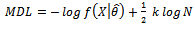 | (5) |
To apply the information theoretic criteria to detect the number of signals, we can say that[16]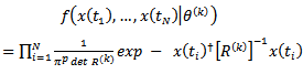 | (6) |
Taking the logarithm and omitting terms that do not depend on the parameter vector  , we find the log-likelihood function
  as
as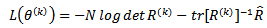 | (7) |
The maximum-likelihood estimate is the value of  that maximizes (7). These estimates are
  | (8a) |
 | (8b) |
 | (8c) |
Substituting the maximum likelihood estimates (8) in the log-likelihood (7), with some straightforward manipulations, we obtain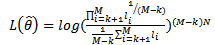 | (9) |
The form of AIC for this problem is therefore given by equation (10).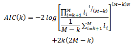 | (10) |
while the MDL criterion is given by equation (11).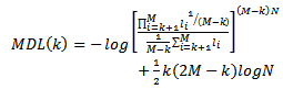 | (11) |
The number of signals  is determined as the value of
 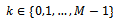 , for which either the AIC or the MDL is minimized[16].
3.2. Estimating the Number of Signals Using EGM
Just like traditional AIC and MDL methods, EGM family also determine the number of non-coherent sources according to the eigenvalues of auto-correlation matrix[8]. The first step is calculating the spatial auto-correlation matrix of the output data  of the sensor array by (3). The second step is applying eigen-decomposition on auto-correlation
  , and arranges the eigenvalues in descending order,
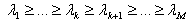 | (12) |
There is a significant difference between  and
and  . So, the number of signal k can be determined by checking the difference between neighbour eigenvalues. This is the main idea of the set of EGM methods. A common used checking method named EGM1[8] is cited as follows:1. Define the average grads of all eigenvalues by
 | (13) |
2. Calculate the gradients of all neighbor eigenvalues as | (14) |
3. Find out all  satisfying
  to construct the set
  . 4. Take the
  that is the first one of the last continuous block of
  in the set
  , and the estimated number of signals is
  .
.
3.3. Simulation of Non-Coherent Signals
Computer simulations have been carried out to examine the effectiveness of above mentioned algorithms in the case of non-coherent sources. Detection probability is the performance metric to evaluate and also compare MDL, AIC and EGM algorithms.The performance of determining the number of non-coherent sources with MDL, AIC and EGM under different SNRs is evaluated in the first experiment. In this experiment, the uniform linear array with 10 sensors is used, element spacing is half-wavelength and SNR is define as | (15) |
Two non-coherent signals with equal powers impinge on the array at  and
and  , SNR changes from
  to
to with step size
  and the number of snapshots is
  . For each SNR,
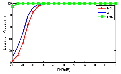
  Monte Carlo trials are run to find probability of success.In Fig. 1, the probabilities of detection for MDL and AIC are compared with EGM in the case of non-coherent sources. According to this Figure, for SNRs lower than
  , the performance of EGM is better than both MDL and AIC methods. For higher SNRs, greater than
  , MDL and EGM show
  success but AIC offers detection probability a bit lower than
  .
.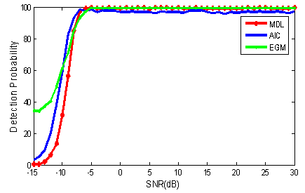 | Figure 1. The detection probability versus SNR for experiment 1 |
In the second experiment, the performance of determining the number of non-coherent sources using MDL, AIC and EGM under different distances between source angles is evaluated. In this case, the uniform linear array with 8 sensors is used. Two non-coherent signals with equal powers impinge on the array, the angular distance changes from 1 to 10 degrees and the number of snapshots is 100. The simulation results of experiment 2 are shown in Fig. 2. As depicted in this figure, in small differences between the incident angles (lower than  ), MDL and AIC have a much better detection performance than EGM. In addition, for differences lower than
  , EGM performance degrades drastically. In the other hand, MDL and AIC performance will be decreased for the angular differences lower than
  Moreover, for the differences greater than
  , EGM is a much better than MDL and also AIC.
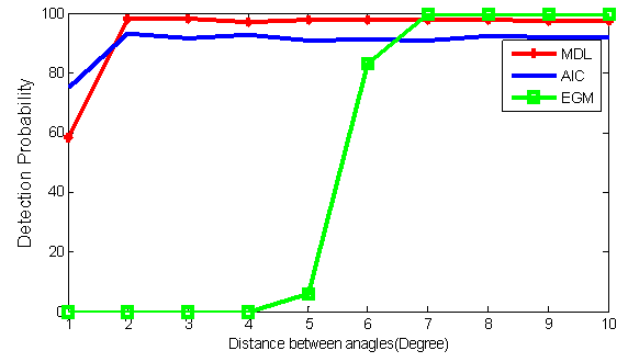 | Figure 2. The detection probability versus different angular differences for experiment 2 |
4. Determining the Number of Coherent/Correlated Sources
A major problem with above methods (MDL, AIC and EGM) is that, they are not applicable to the case of fully correlated signals, referred to as the coherent signals. This case appears especially in multipath propagation and therefore it is of great practical importance. In this investigation, we focused on spatial smoothing method to solve the coherency/correlation, and then the number of coherent sources is estimated considering the pre-processed output signal of array antenna.The spatial smoothing scheme first suggested by Evans and extensively studied by Shan[14]. Their solution is based on a pre-processing scheme that divides the total array of sensors into overlapped sub-arrays and then, generates the average of the sub-array output covariance matrices. This forward-only smoothing scheme makes use of a larger number of sensor elements than the conventional ones, and in particular requires  sensor elements to estimate any
  directions of arrival. In[15], it is proved that by simultaneous use of a set of forward and complex conjugated backward sub-arrays, it is always possible to estimate any
  directions of arrival using at most[
 ] sensor elements. So, in this research work, we pre-processed coherent signals using FBSS as the first step of the process of determining the number of coherent sources.
4.1. Forward/Backward Spatial Smoothing Technique for Coherent/Correlated Signal Identification
FBSS scheme starts by dividing a uniform linear array with  sensors into uniformly overlapping sub-arrays of size
  (see Fig. 3). Let
  stands for the output of the
  th sub-array for
 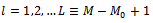 where L denotes the total number of these forward sub-arrays[15].
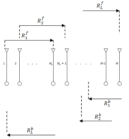 | Figure 3. The forward/backward sub-arrays in FBSS scheme[15] |
 | (16) |
Then, the covariance matrix of the  th sub-array is given by
 | (17) |
Forward spatially smoothed covariance matrix  as the mean of the forward sub-array covariance matrices is
  | (18) |
The covariance matrix of the  th backward sub-array is given by
 | (19) |
In the same way as (18), the spatially smoothed backward sub-array covariance matrix  is
is | (20) |
Finally, the forward/backward smoothed covariance matrix  as the mean of
  and
and  is given by
 | (21) |
Since the smoothed covariance matrix  in (21) has exactly the same form as the covariance matrix for some non-coherent situations, the eigenstructure-based techniques can be applied to this smoothed covariance matrix to successfully estimate the number of coherent sources[15].
4.2. Simulation of Coherent/Correlated Sources
Computer simulations have been carried out to examine the effectiveness of above mentioned algorithms in coherent case. An uniform linear array with 9 sensors is used, SNR changes from  with step size 1 dB and the number of snapshots is
  . For each SNR,
  Monte Carlo trials are run.As the experiment 3, the performance of FBSS-based MDL, AIC and EGM algorithms under different SNRs for coherent sources is investigated. Three coherent signals with equal powers impinge on array at
  are considered with the path coefficients
  ,
, 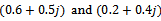 , respectively. As depicted in Fig. 4, for SNRs greater than
  , the performance of EGM is better than MDL and AIC methods but in SNRs lower than
  , none of methods can detect the number of coherent sources.
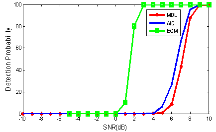 | Figure 4. The detection probability versus SNR for experiment 3 |
In experiment 4, signal sources are considered as correlated non-coherent ones. Three correlated signals with equal powers impinge on array at  and
and  Correlated signals are obtained by filtering the signal through a first order auto-recursive (AR1) filter, given by
 | (22) |
where  is the correlation coefficient. In this experiment
  is assumed. Simulation results are shown in Fig. 5. In this case, FBSS-based methods can effectively detect the number of sources and offer high detection probabilities even much better than experiment 3. According to Fig. 5, EGM offers higher performance with respect to MDL and AIC methods. As a highlighted remark, EGM method shows high detection probability for low SNRs (lower than
  ).
). | Figure 5. The detection probability versus SNR for experiment 4 |
5. Conclusions
In this paper, we focused on the performance evaluation of three popular methods, AIC, MDL as well as EGM. As shown in simulation results, these algorithms are appropriate for determining the number of non-coherent signals and the performance of them will be decreased when signals are coherent and/or correlated. A solution to this problem, applicable to coherent as well as correlated non-coherent sources, is to use spatial smoothing method to solve the coherency or correlation, and then estimating the number of signals.Computer simulations showed that, in the case of non-coherent signals, in low SNRs, EGM is better than MDL and AIC. Also, in small angular differences, MDL and AIC algorithms offer a higher detection performance with respect to EGM.Moreover, simulation results for FBSS-based algorithms, in the case of coherent sources as well as correlated ones, showed the higher detection probability for EGM compared to AIC and MDL. In this research we compared MDL, AIC and EGM algorithms in additive white Gaussian noise (AWGN) channel. Eigen increment threshold (EIT) method which is proposed as a method to determine the number of sources can be researched in AWGN channel and compared to AIC, MDL and EGM algorithms in both non-coherent and coherent cases. In addition, these methods can be investigated in colored noise scenario and in the case that exist different groups of non-coherent sources containing coherent signals. Modeling and determining the number of sources with unequal powers is another new research work to be done in this field.
ACKNOWLEDGEMENTS
This work has been supported by Research Institute for ICT (ITRC) under contract number 19248/500 (28.12.1390).
References
| [1] | S. Shirvani Moghaddam, S. Almasi Monfared, “A Comprehensive Performance Study of Narrowband DOA Estimation Algorithms,” International Journal on Communications Antenna and Propagation (IRECAP), Vol. 1, No. 4, pp. 396-405, August 2011. |
| [2] | S. Valaee, P. Kabal, “An Information Theoretic Approach to Source Enumeration in Array Signal Processing,” IEEE Trans. Signal Processing, Vol. 52, No. 5, pp. 1171–1178, May 2004. |
| [3] | J. Liu, J. Xin, N. Zheng, and A. Sano, “Detection of the Number of Coherent Narrowband Signals with L-Shaped Sensor Array,” IEEE 10th International Conference on Signal Processing (ICSP), pp. 323-326, Oct. 2010. |
| [4] | J. Jiang, M. Ann Ingram, “Robust Detection of Number of Sources Using the Transformed Rotational Matrix,” IEEE Wireless Communications and Networking Conference (WCNC’04), Vol. 1, pp. 501-506, March 2004. |
| [5] | D.B. Williams, “Detection: Determining the Number of Sources,” Digital Signal Processing Handbook, Chapter 67, CRC Press LCC, 1999. |
| [6] | L. Huang, S. Wu, “Low-complexity MDL Method for Accurate Source Enumeration,” IEEE Signal Processing Letters, Vol. 14, No. 4, pp.581–584, Sep. 2007. |
| [7] | L. Huang, T. Long, E. Mao and H. C. So, “MMSE-based MDL Method for Accurate Source Number Estimation,” IEEE Signal Processing Letters, Vol. 16, No. 9, pp. 798-801, Sep. 2009. |
| [8] | Q. Zhang, Y. Yin, and J. Huang, “Detecting the Number of Sources Using Modified EGM,” IEEE Region 10 Conference (TENCON), pp. 1-4, Nov. 2006. |
| [9] | F. Chu, J. Huang, M.Jiang, Q. Zhang, and T. Ma, “Detecting the Number of Sources Using Modified EIT,” 4th IEEE Conference on Industrial Electronics and Applications (ICIEA), pp. 563-566, May 2009. |
| [10] | J. Zhen, X. Si, and L. Liu, “Method for Determining Number of Coherent Signals in the Presence of Colored Noise,” Journal of Systems Engineering and Electronics, Vol. 21, No. 1, pp. 27–30, February 2010. |
| [11] | L. Jing-hua, L. Rong, “Source Number Detection in Spatial Correlated Color Noise Using the Canonical Correlation Coefficients,” 4th IEEE Conference on Industrial Electronics and Applications (ICIEA), pp. 1597-1601, May 2009. |
| [12] | S. Yi, H. Sen, and T. Liang-Rui,” A new Estimation Method Based on Feature Difference for Coherent Source,” 6th International Conference on Wireless Communications Networking and Mobile Computing (WICOM), pp. 1-4, Sept 2010. |
| [13] | M. Wax, I. Ziskind, “Detection of the Number of Coherent Signals by the MDL Principle,” IEEE Trans. Acoustics, Speech, and Signal Processing, Vol. 37, No. 8, pp. 1190-1196, Aug. 1989. |
| [14] | T.J. Shan, M. Wax, and T. Kailath, “On Spatial Smoothing of Estimation of Coherent Signals,” IEEE Trans. Acoustics, Speech, Signal Processing, Vol. 33, No. 4, pp. 806-811, 1985. |
| [15] | S.U. Pillai, B.H. Kwon, “Forward/Backward Spatial Smoothing Techniques for Coherent Signals Identification,” IEEE Trans. Acoustics, Speech, Signal Processing, Vol. 37, No. 1, pp. 8-15, 1989. |
| [16] | M. Wax, T. Kailath, “Detection of Signals by Information Theoretic Criteria,” IEEE Trans. Acoustics, Speech, Signal Processing, Vol. 33, No. 2, pp. 387–392, Apr. 1985. |
 Abstract
 Reference
 Full-Text PDF
 Full-Text HTML