1. Introduction

Computer simulation has become a useful part of modeling many natural systems in physics, chemistry and biology, and human systems in economics and social science (the computational sociology) as well as in engineering to gain insight into the operation of those systems. A good example of the usefulness of using computers to simulate can be found in the field of network traffic simulation. In such simulations, the model behavior will change each simulation according to the set of initial parameters assumed for the environment[1-3]. Traditionally, the formal modeling of systems has been via a mathematical model, which attempts to find analytical solutions enabling the prediction of the behavior of the system from a set of parameters and initial conditions. Computer simulation is often used as an adjunct to, or substitution for, modeling systems for which simple closed form analytic solutions are not possible. There are many different types of computer simulation; the common feature they all share is the attempt to generate a sample of representative scenarios for a model in which a complete enumeration of all possible states would be prohibitive or impossible.

Several software packages exist for running computer- based simulation modeling (e.g. Monte Carlo simulation and stochastic modeling) that makes the modeling almost effortless. Modern usage of the term ‘computer simulation’ may encompass virtually any computer-based representation.

1.1. Purposes of Simulation

The simulation modeling and analysis of different types of systems are conducted for the purposes of[5]:

· Gaining insight into the operation of a system

· Developing operating or resource policies to improve system performance

· Testing new concepts and/or systems before implementation

· Gaining information without disturbing the actual system

Computer simulation has the potential to revolutionize the development process in the field of non-woven industry. The great advantage of manmade fiber is their design ability uniformity. Based on these properties, non-woven parameters such as porosity, fiber thickness distribution, fiber orientation and porosity gradient s are to a large extent at the command of the experienced non-woven manufacturer. The problem is generally the cost of trying out new parameter sets, lab scale production often does not completely agree with production scale non-woven and stopping the production lines for parameters studies is very costly. Computer simulation can reduce the number of trail runs of producing new material prototypes significantly[6-7]. They help understanding the production processes as well as the functionality of the non-woven and may point out trends or improvements that would be costly to find using traditional methods. So instead of producing many candidate materials and choosing the best one afterwards, the simulation yields suggestions for a very good candidate beforehand.

1.2. Advantages to Simulation

In addition to the capabilities, simulation modeling has specific benefits. These include[8];

· Experimentation in compressed time

· Reduced analytic requirements

· Easily demonstrated models

2. Important Elements for Simulation of Non-woven

3. Principle of Simulation

A Non-woven model is produced based on the fiber type, fiber length distribution, diameter, crimp, orientation; maximum allowed bending angle and porosity of the structure required etc. The porosity is mainly governed by the number of fibers. First the fibers are considered as a long thick and flexible and in simple case the fiber is allowed to fall on a previously laid fiber or on a platform. While allowing the fiber to fall on a previously laid layer, the new fiber is seated on a previously laid fiber[8-9], if the part of the fiber is not found any fiber of this layer it will try to bend some more distance to find a support. In a real model simulation the image of the real non-woven structure is considered.

3.1. Steps for Simulation of Non-woven Structures

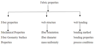
[A] Web

· Fiber properties – diameter, length, variability

· Structure properties – Orientation Distribution Function (ODF), thickness, layers, variability[9-10]

[B] Bonding

· Thermal bonding (Calendar and Thru-air)

· Mechanical (Needling and Hydro entangling)[10,11]

[C] Modeling Performance

Fiber thickness or fiber shapes, fiber diameter and porosity are comparatively easy to determine. Much harder is the estimation of fiber orientation. In a simple non-woven model is developed based on the assumptions that the portion of the non-woven that can be represented in the computer memory is small compared to fiber length and fiber crimp. So the orientation of the fiber segment in a non-woven is entered as an input from the past data [12].

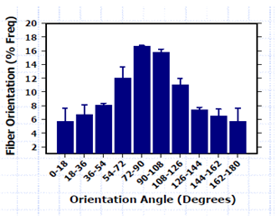Figure 1. Orientation angle Vs fiber orientation (%frequency) [12]

To reproduce existing media, the grammage and specific weight of the fiber material can be used to infer the porosity from the thickness of the non-woven. Manufacturers usually know the types of fibers they use, so the only difficulty lies in establishing the orientation. So the orientation angle and their frequency percentage are estimated from the real fabric model and it is feed as an input.

3.2. Simulation Algorithm

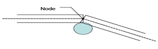
The fibers in the web are modeled by cylinders linked together by the hereon-called ‘nodes’ around which they can freely rotate in the z-direction (as in pivots). In order to generate a 3-D fiber web, horizontal straight fibers are sequentially dropped on a forming surface or previously deposited fibers. In other word, when a new horizontal fiber is generated, both the web and the new fiber are projected onto the forming surface. A subset of the web is created from the projected fibers that intersect the projection of the new fiber. This subset will be used instead of the full web in order to speed up the computations. If there are no fibers underneath the new one, it will be directly placed on the forming surface and the procedure will restart. However, if the new fiber is likely to hit fibers from the web, the next step is to lower the new fiber on the web (i.e., to find the smallest vertical translation which will bring the new fiber in contact with the web) as shown in figure[13].

Figure 2. Schematic of web generation algorithm[13]

If there are several occurrences of a smallest value, all of the corresponding impact points are used; when a fiber falls on an existing fiber, a new node is generated on its axis and the fiber is split into two segments. Our algorithm allows for these new fiber segments[5] to rotate downward around this node, emulating bending of the original fiber over the deposited one at the crossover. When the two segments rotate around their common node, small parts of them get inside the existing fiber as well as each other as shown in the figure.

Figure 3. Fiber interactions at a contact point[13]

3.3. Methods of Non Woven Structure Simulation

[a] Virtual generation

[b] Obtaining structure from the real model

Starting point of the web structure simulation is the construction of the three dimensional microscopic model of the non-woven. Such a model can be obtained either from an image of the non-woven (DVI, tomography, etc), or by virtually generating a three dimensional model[14]. While real images might be used when comparing measurement and simulation, computer generated models are necessary when designing new materials. In addition to the cost of acquiring the three dimensional image, the final influence of image processing procedures used to obtain a binary image from a real non-woven must be considered.

3.4. Virtual Generation

The input parameters to be given for creating a virtual web generation are:

· Porosity

· Fiber orientation distribution (anisotropy)

· Fiber diameter (distribution)

· Fiber cross sectional shape

· Fiber length (distribution)

The following fig 4 shows the generated non-woven fiber structure with a size of 512µm x 512 µm x 128 µm, and an overall porosity of 82 %[3]. The resolution is 1µm per voxel. The fibers have a circular cross section, a diameter of 7 µm, and are oriented along the x-y plane 3D Web Generation - Dropping Fibers on the Web. The following fig shows the simulation of web generation[7-8,15].

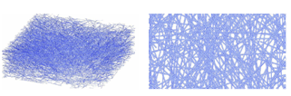Figure 4. 3D simulation Web generated by virtual generation[8]

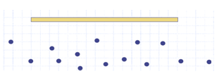Figure 5. The new fiber is created above the web[8]

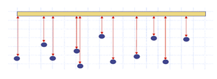Figure 6. The distance between the new fiber and web are computed[8]

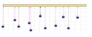Figure 7. Smallest one is selected[8]

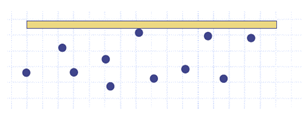Figure 8. New fiber is lowered to contact[8]

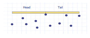Figure 9. The new fiber is split into head and tail[3]

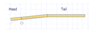
Figure 10. The bending angles are computed[15]

Figure 11. The smallest angle is selected[15]

Figure 12. The head is now shorter, and the process is restarted[7]

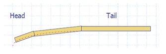Figure 13. No more fibers under the head, the head follows the bending profile The process is finished for the head[7]

4. Simulation Obtained From the Real Model

First, images of the microstructure of the material have to be obtained. For a wide range of materials, this can be achieved by computer tomography using X-ray absorption contrast (XCT). Unfortunately, materials with low absorption contrast and fine structures do not yield the necessary image quality when using XCT[16]. New 3D imaging techniques like phase contrast tomography relying on the use of synchrotron radiation overcome this problem. However, 2D microscopic images of cross-sections are still cheaper, faster, and with less effort to get. After the image acquisition, a model from stochastic geometry is adapted to the microstructure by fitting the model parameters. To this end, geometric characteristics of the microstructure are determined and the parameters of the model are chosen such that characteristic properties of the material (e.g. porosity or fiber radius distribution) are represented correctly for suitable methods[7,8].

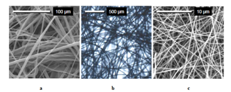Figure 14. Microscopic images of a) Meltblown, b) Spunbonded and c) Electro-spun fiber-webs shows the microscopic images of the various typical non-woven structures made by melt blown, spunbonded and electro spun fibers web[7]

5. Computer Simulations for Filtration: Layered Media Model

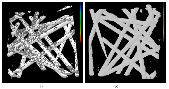
The first ingredient in the simulation of air filtration is a three-dimensional representation of the filter media in the computer used a voxel model, where a large enough cutout of the media is discretized by a uniform Cartesian grid with edge-length h. This h has to be chosen in such a way that the grid resolves the smallest occurring fiber diameter. For example, for smallest fiber radius in the non-woven 5µm, h = 2.5 µm will resolve this fiber with 4 voxels per diameter. This introduces the next parameter in the model: the side lengths of the cutout. The cutout must be large enough to model a representative portion of the media. On the other hand, available computer memory limits the size of the cutout. A third consideration is that the thickness of the filter media should be resolved completely. Thus, if the media is 2 mm thick and a voxel is 2.5µm, then about 840 voxels are needed in the flow direction including a little empty space before and after the media. Then the capability to compute the air flow and particle motion through the geometry limits the extent of the lateral directions. Under the restrictions on the computationally feasible cutout, the fibers may often be modeled as straight and infinitely long; for example when the fiber is say 7cm long with two revolutions per 10 cm but the longest edge of the cutout is 2mm. The model is then complete after choosing the porosity of the media and the anisotropy of the fibers[2]. Usually, the air flows perpendicularly to the machine direction, which is also the main anisotropy. Think of it as the Z-direction of the model. Last but not least, the porosity is prescribed. For filter media layers it ranges between 80% to 98% porosity. To build a virtual non-woven, here create random fiber positions, fiber types and fiber directions. The position is uniformly distributed in the cutout; the fiber type is drawn according to its probability, and the fiber direction according to the choice of anisotropy[16]. This fiber is discretized into voxels and entered into the domain, with the option to overlap or not overlap with previously entered fibers. This procedure is repeated until the percentage of voxels not covered by fibers is lower than the desired porosity. If the achieved porosity is too far from the desired one, the procedure is repeated in the hope to find by chance a configuration that satisfies the porosity requiremen[4,7]. However, for large enough domain it is usually not a problem to achieve less than 1% deviation from the desired porosity. Finally, two or more of these layers can be stacked to achieve a realistic representation of layered filter media. Two highly porous layers are chosen not to represent a real air filter media (where at least one layer of lower porosity should be present) but for the sake of clear differentiation and three-dimensional view of the media.

6. Flow Simulation

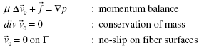
Stefan Rief, Arnulf Latzand Andreas Wiegmann, consider low Reynolds numbers typical for some air filtration processes and solve the Stokes equations with periodic boundary conditions[9]:

To drive the flow, a constant body force in the z-direction is applied. Through periodicity, artificial fiber ends are felt by the flow on the cutout surfaces in the x- and y-directions where a fiber ends on the opposite cutout surface. This influence is another reason why a large enough cutout must be used in the computations. The three components of the velocity v as well as the fluid pressure p are all available at voxel centers after the calculations, with zero-values assigned inside the fiber voxels.

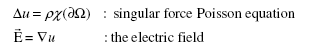
7. Model of Surface Charges and Computation of Electric Field

The charges are assumed as constant given forces on the fiber surfaces, the fiber voxel walls that neighbor fluid voxels. For the moment, a single constant amount of charge r is assigned on all such voxel walls. The following boundary value problem is solved for the potential[1]:

Here u is periodic in the x- and y-directions, and satisfies zero Dirichlet boundary conditions on the boundaries at –Z₀ and nZ + Z₀ in the z-direction. By construction, these boundaries lie away from the fibers and there is no conflict between singular forces on fiber surfaces and these Dirichlet conditions[15,17]. Due to the periodic boundary conditions, the potential feels a non integrable amount of charges, and tends to infinity in the non-woven as the Dirichlet boundary is moved away from the non-woven. That is, the potential u depends on the position where the Dirichlet condition is located. However, the electrical field E remains almost unchanged from the location of the Dirichlet boundary as soon as this boundary is sufficiently far away from the non-woven. This electric field enters in the equation of motion for the particles together with the charges on the particles as described in the next section[9].

Figure 15. Deposition of particles on fibers in porous layer[9]

Particle sizes are distributed according to the fine test dust. They are deposited at random positions in a plane perpendicular to the flow direction and then to their deposition locations by the stochastic ODE (a) front view and (b) rear view.

8. Measurement v/s Simulation in Filtration

As mercury is non-wetting to most materials, intrusion of mercury into pores only occurs when pressure is applied on the mercury. In the experimental setup the pressure on the mercury is subsequently raised, and the volume of the intruding mercury (which equals the volume of the intruded pores) is measured. The pressure p is related to the pore radius r via; The Young-Laplace equation[3]:

ρ = 2γcosθ/ r

Where is the surface tension and the contact angle of mercury. Thus, a size distribution of pores is determined. This method cannot measure the volume of closed pores. Furthermore, large pores hidden behind smaller bottlenecks are not filled with mercury until the pressure is high besides mercury intrusion porosimetry, also considers geometrical pore size distributions and liquid extrusion porosimetry[18]. The differences between the different methods are significant, just as in real measurements, and illustrated in Figure 3. The studies in the next sections could be equally well performed on these other measures of pore sizes if needed for agreement with real measurements.

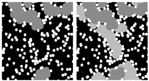Figure 16. Two dimensional view illustrating the method of a mercury intrusion porosimetry simulation[18]

Fibers are white, and grey areas indicate pores of radius r ≥ 20 and r ≥ 16, respectively. All marked pores are always connected to one of the mercury reservoirs on top or bottom of the sample by a wide enough paths.

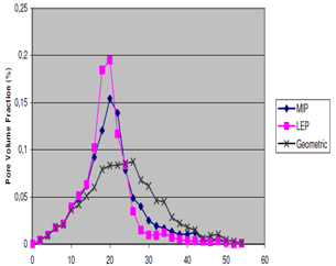Figure 17. Pore size distribution Vs Pore volume fraction (%)[19]

The diagram shows the calculated geometric pore size distribution and the results of the simulated mercury intrusion porosimetry (MIP) and the simulated liquid extrusion porosimetry (LEP)[19].

9. Simulation to Measure the Mechanical Properties

Instead of treating the distortion of the fabric by a fine deformation approach in which individual fiber strains are related to the fabric strain, more microscopic treatment of individual bond sites have focused. This simulation is thus reminiscent of the molecular dynamics description of a, fluid which is based on the motions of the individual units of the system. Requiring, each bond site to be in static equilibrium for a given set of external constraints leads to a determination of the position of each of the sites. Knowledge of site positions approach in which individual fiber a fabric would consist of say a rectangular area which, when replicated in two directions, reproduces the appearance of the fabric in the large. The sample size must be sufficiently large, consisting of at least several hundred bond sites, in order to possess the same mechanical properties as a macroscopic sample used in the laboratory. The optimum number of bond sites to consider will depend on a balance between the degree of faithful representation of the fabric desired and the attendant increase in computing time[4]. While not yet investigated this aspect, one criterion must certainly be met. Two macroscopically identical samples (differing only in microscopic detail) must have essentially the same bulk mechanical properties. The ingredients described above are fed into the main program which carries out the analysis of the system when one or more boundaries are subjected to specified distortions. For example, one lateral boundary of a rectangular planar sample may be (mathematically) displaced by an incremental amount while the opposite parallel boundary remains stationary. The two remaining boundaries are left free to. Move and will find new positions in accordance with the laws of physics here are concurrent forces acting at each intersection of two or more fibers, but each such point is in static equilibrium. Thus at each bond site, the requirement of static equilibrium is that ∑ Fi = 0; where the forces are those exerted on a bond site by each of the fiber segments[5-7].

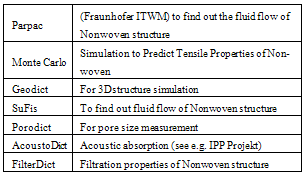
10. Commercial Software Used for Nonwoven Structure Simulation

The following are the some the commercialized software used in the Nonwoven industry [4-7,17].

11. Disadvantages to Simulation

Although simulation has many advantages, there are also some disadvantages of which the simulation practitioner should be aware. These disadvantages are not really directly associated with the modeling and analysis of a system but rather with the expectations associated with simulation projects. These disadvantages include the following [9]:

· Simulation cannot give accurate results when the input data are inaccurate.

· Simulation cannot provide easy answers to complex problems.

· Simulation cannot solve problems by itself

12. Conclusions

It is clearly shows that the simulation process has the great potential in the non woven industry. The simulation of non woven structure has ability to measure or predicting the end use of that material without much time coat. It also does not require much skill after developing the model.