Ketcheuzeu-Ngakam J.1, Koueni-Toko C.2, Djeumako B.1, Tcheukam-Toko D.3, Kuitche A.4
1Department of Mechanical Engineering, ENSAI, University of NGaoundéré, N’Déré, Cameroon
2Department of Renewable Energy, ISS, University of Maroua, Maroua, Cameroon
3Department of Energy Engineering, IUT, University of NGaoundéré, P NGaoundéré, Cameroon
4Department of Electrical, Energy and Automatism Control Engineering, ENSAI, N’Dere, CMR
Correspondence to: Tcheukam-Toko D., Department of Energy Engineering, IUT, University of NGaoundéré, P NGaoundéré, Cameroon.
| Email: |  |
Copyright © 2014 Scientific & Academic Publishing. All Rights Reserved.
Abstract
Numerical analysis was performed for a flow in a Kaplan turbine placed inside a pressure pipe of a hydroelectric dam. Special attention has been paid for the friction effect and the vortexes structures through the flow inside the volute, the distributor and the runner. The turbulent model has been applied a standard κ-ω two equations model and the two-dimensional Reynolds Averaged Navier–Stokes (RANS) equations, are discredited with the second order upwind scheme. The SIMPLE algorithm, which is developed using control volumes, is adopted as the numerical procedure. Calculations were performed for a wide variation of Reynolds numbers. The results reveal that with increasing of Reynolds number, the height of vortexes increases inside the discharge rings and blades, accelerating the detachment of the boundary layer. Comparison of numerical results with the experimental data available in the literature is satisfactory.
Keywords:
Kaplan turbine, Hydrodynamic parameters, Runner, Dynamic field, Hydroelectricity, CFD
Cite this paper: Ketcheuzeu-Ngakam J., Koueni-Toko C., Djeumako B., Tcheukam-Toko D., Kuitche A., Characterization of Hydrodynamics Parameters of a Kaplan Turbine, Energy and Power, Vol. 4 No. 3, 2014, pp. 58-69. doi: 10.5923/j.ep.20140403.03.
1. Introduction
In worldwide production of electricity, the hydraulic part is always in expansion (2% per year average). This option produces annually 2740 TWH from a power installed of 800 GW. More than 94% of installations have a power of more than 10 MW, and have hence taken the name of “Big Hydroelectric Center”. Following the yearly climatic condition, the production of electricity coming from the hydraulic, represents 16 to 18% of worldwide production according to Duprat [1]. This figure makes the hydroelectricity one of the most contributing significant actually in the renewable energy sources.This electricity is produced by an important mechanic dispositive called hydraulic turbine. It’s is used to transform potential energy and the kinetic energy of water, in mechanic energy. This will then be transformed into electric energy by an alternator. There exist two categories of hydraulics turbine. The turbine of action, which does not constitute a draft tube and functions with the kinetic energy of water, and the turbine of reaction, which functions with the pressure difference and the energy pressure. With the increasing coast of energy and the high demand of green energy, hydraulic turbine of thin height of falls such as Francis and Kaplan turbines, are those targeted as being economically profitable. They are constituted of distributor, volute, runner and draft tube. The runner is a mechanic dispositive which is used to recuperate all the energy as mechanic energy and transfer it to a generator which provides electrical energy.Many studies on the flow in the Kaplan turbine have been done. Liu et al. [2], have summarized the results of the simulation of unstable flow in a Kaplan turbine with a rotor diameter of 350 mm. This result has been employed to analyze the hydraulic stability and the performances of the turbine. Liu et al. [3], have then proved that the prevision of the pressure fluctuation at different positions along the flow passage is conformed to the experimental data, in terms of frequency and amplitude. They have carried out an experimental study on the prototype of turbine in a hydraulic center. They showed that the intense abnormal oscillation is produced during the closure of discharge rings. The frequency of this intense oscillation is of 1.05 the rotation frequency of the rotor. They have effectuated simulations by using the calculation of the interaction of fluid-structure, with a specified model. This study has permitted to show that there is a strong possibility of having resonance between the frequency of rotor rotation and the intrinsic frequency of the water body. Petit et al. [4], have carried out a numerical study of a stationary flow through different components of a big Kaplan turbine of prototype and compared the results with those using a different program. Zhou et al. [5], have carried out the simulation in turbulent regime of an unsteady flow passing the complete way of a flow in a Kaplan turbine prototype at many functioning conditions. They did not clarify the origin of the abnormal intense oscillation at certain frequency of the rotor rotation. Merahi et al. [6], carried out a numerical study of a three dimensional stationary and incompressible flow through the blades system of a runner, with the help of a code FAST3D, by using the k-ε model. They showed that loses due to the variety of the incidence angle are considered like the principal cause of the decrease in efficiency of turbo machinery. Hilgenfeld et al. [7], have carried out an experimental study on the flow in the Kaplan turbine and showed the wake effects on the development of boundary layer during the flow passage through the blades system of a runner. Behanu [8], has carried out experimental measurements of the velocity by using the LDV with corresponding values of RMS for an inclination of distributors of 26° and 32°. They concluded that the RMS values were very important at the level of the turbine rotor because of the rotation of this one. They observed the zones of low velocity at the level of the rotor cone. We observed that the hydrodynamics parameters act with the flow oscillatory and flow linearity, which justifies the necessity to study their influences on the efficiency of the Kaplan turbine.This present work consists in doing a numerical study of dynamic field of a flow in a Kaplan turbine. A special attention will be paid on the flow through these three principal elements of turbine: volute, distributor or discharge rings, and runner/blades: This study would help to well understand the influence of hydrodynamic parameters on the efficiency of the Kaplan turbine. To lead well this study, we are going to present the mathematical formulation and the computation procedure employed. These methods have permitted to calculate, the velocity and pressure fields in the volute and runner of the Kaplan turbine, and the velocity profiles at the entrance of volute, by using a model of bi-dimensional turbulence, isotropic and stationary k-ω model.
2. Mathematical Formulation and Computation Procedure
2.1. Assumption of Calculation Domain
Our work of simulation is done through a volute, a distributor and a runner of Kaplan turbine placed inside a pressure pipe of a hydroelectric dam. The geometry and the dimensions of the Kaplan turbine have been chosen in conformity with the experimental works of Behanu [8]. He carried out his experimental study at Hölleforsen (Swede), hydroelectric station. This station is situated on the Indalsäven River in Swede. It’s consisted of three unities of Kaplan turbine having 50 MW of total capacity installed. The operational dimension of the head is 27 m, with a rotor diameter of 5.5 m each one, and a discharge capacity of 230 m3/s for each turbine. The measures have been carried out on a reduced model of 1:11 scale of the Kaplan turbine represented by the figure 1 bellow. The rotor diameter is 500 mm, its velocity is 595 rpm, and the rate of flow is 0.522 m3/s. This work condition is near the best possible efficiency with an operational head of 4.5 m for a load of 60%. The pressure pipe carries water flow at high pressure from the upstream basin to the suction port. This flow on high pressure is responsible of velocity profiles obtained at the entrance of the volute.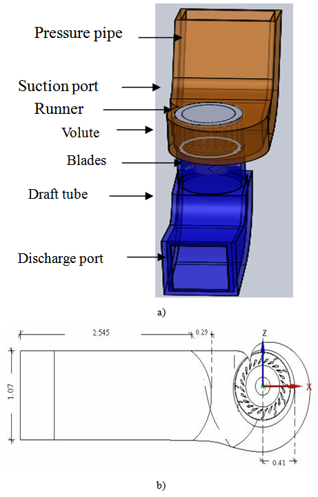 | Figure 1. Geometry and dimensions of the Kaplan turbine (Behanu [8]); a): Kaplan turbine; b): runner casing dimensions |
2.2. Governing Equations
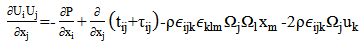
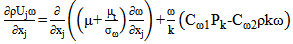
The monophasic turbulent flow in the Kaplan turbine is described by a set of non-linear partial differential equations expressing the physical laws of conservation between the velocity and pressure at each point of the flow: the Navier-Stokes equations. To these equations, we add the equation of turbulent kinetic energy and that of its dissipation rate like proposed by Launder and Spalding [9]. Solving these equations will reveal features such as pressure and dynamic fields, and axial/tangential velocity profiles. | (1) |
 | (2) |
The relation (1) is a continuity equation, and (2) is the equation of the quantity of movement conservation in which:• the left term represents the convective transport;• the first term on the right represents the forces due to the pressure;• the second term on the right represents the forces of viscosities;• the third term on the right represents the centrifugal term,• the fourth term on the right represents the Coriolis term are given by the relations:
 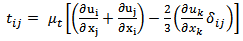 | (3) |
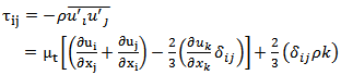 | (4) |
These relations have been replaced in the relation (2), to obtain the relation (5) bellow.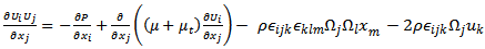 | (5) |
Because of the potential, gravitational and centrifugal nature of the pressure, the gradient of reduced pressure is given by the relation (6) bellow.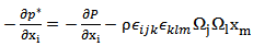 | (6) |
While the reduced pressure P* is given by: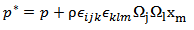 | (7) |
The Wilson [10],  model for the turbulent kinetic energy k and the specific dissipative rate
  is given by the relations (8) and (9) bellow.
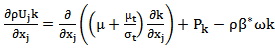 | (8) |
 | (9) |
Where the turbulent viscosity µt, and the production terms are given respectively by the relations (10) and (11) bellow. | (10) |
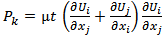 | (11) |
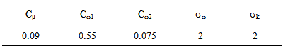
Where, Cµ, Cω1, and Cω2, are empirical constants; σω and σk are respectively the turbulent Prandtl numbers relative to ω and k. The values of these constants proposed by Jones and Launder [11], are represented on table 2 bellow.Table 2. Empirical constants proposed by Jones and Launder [11]
 |
| |
|
At the walls, a no-slip condition is applied for a velocity corresponding to the value of k = 0 and at the first node perpendicularly to the wall at: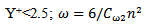 | (12) |
Where, n represents the normal distance to the wall. For the pressure at all boundaries, we have the relation (13) bellow: | (13) |
2.3. Computation Procedure
The transition from physical domain to the numerical domain begins with the generating mesh geometry by a preprocessor. Then import this into a computational code for the iterative solution of equations to determine the values of variables on each node of the mesh. The segregated solution method was chosen for the resolution of turbulence model and governing equations. Governing equations were discredited with the control volume technique. For the convective and the diffusive terms, a second order upwind method was used while the SIMPLE (Semi Implicit Method for Pressure Linked Equations) procedure was introduced for the velocity-pressure (Patankar, [12]). The convergence of the numerical calculation is checked by examining the evolution of relative residuals in each governing equation for a convergence criterion of 0.001%. The stability of the iterative process was carried out by relaxation coefficients associated with the velocity, pressure, κ, ω and μt. The Standard Wall-Functions were used to take into account the effects of friction near of wall and around distributor and runner. Three mesh distributions have been tested to ensure that the calculated results are grid independent. The similar method was already used by Tcheukam-Toko et al. [13]
3. Results and Discussion
3.1. Generating Mesh Geometry
The figure 2 below represents the computational domain meshed with the code GAMBIT. The grid distribution is a set of quadrilateral cells (uniformly structured mesh). The calculations will use the software Fluent [14]. The mesh is very uniformly fine near of the wall and around the distributor and the runner, where the velocity gradient is large. The grid distribution impacts the computation time and the number of iterations required for the solution converge. The choice of the mesh size of 130,000 cells is a good compromise and the results that will be presented later are those of this mesh size. The no-dimension variables are: | (14) |
 | (15) |
 | (16) |
 | (17) |
 | (18) |
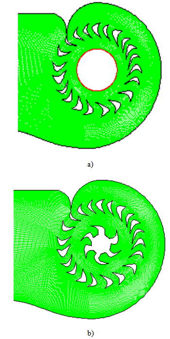 | Figure 2. Grid configuration a): in the volute; b) around the runner |
The no-dimension runner velocity and rate of flow are respectively N+ = 140 and Q+ varying from 0.984 to 0.996.
3.2. Velocity Fields
The figure 3 below represents the axial and tangential velocity fields in the Kaplan turbine volute for different Reynolds numbers. We observe that, the variation of axial velocity is very large around the middle of the volute, which decreases progressively up to the volute wall. The tangential velocity shows a successive variation only at the spiral part of the volute.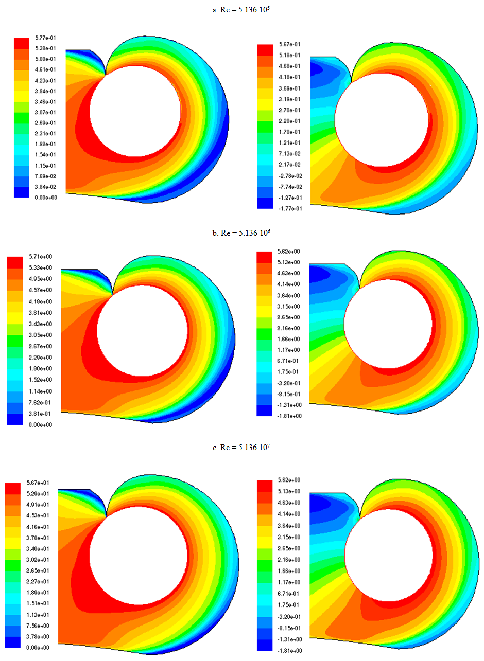 | Figure 3. Velocity fields in the volute Axial velocity (Left column); Tangential velocity(Right column) |
The figure 4 bellow represents the axial and tangential velocity fields in the distributors for differents Reynolds numbers. We observe a boundary layer formation showing an increasing of the axial velocity from the ring axe, and a decreasing of the tangential velocity with the increasing of the Reynolds numbers. This boundary layer inside the discharge ring, allow the recuperation of the kinetic energy. The fluid outing from the discharge ring and reaching the runner will become oscillatory inducing to the runner a centrigugal and Coriolis accelerate rotation mouvement. The oscillatory flow increases and generates many axial and tangential vortex allowing the maximal recuparation of hydraulic energy and then ameliorating the performance of hydroelectric dams.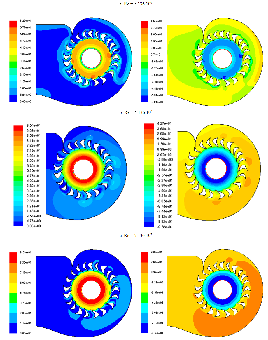 | Figure 4. Velocity fields in the distributors (inlet guides) Axial velocity (Left column); Tangential velocity(Right column) |
The figures 5 bellow represents the velocity field arround the runner for different Reynolds numbers. We observe that, the veloity increases gradually with the Reynolds number and the flow has totally a radial direction. We observe a recirculation zone at the entrance of the runner which shows the presence of vortex characterising a secondary flow.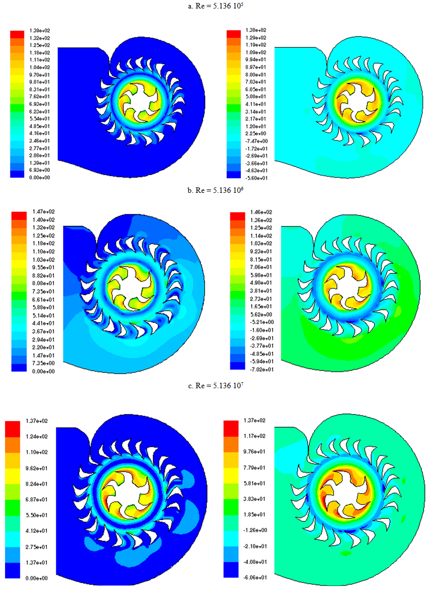 | Figure 5. Velocity fields around the runner Axial velocity (Left column); Tangential velocity(Right column) |
The figure 6 bellow represents the velocity field among the inlet guides of the distributors. We observe that, the velocity is very low at the entrance, and then it increases up to the outlet where it becomes maxima.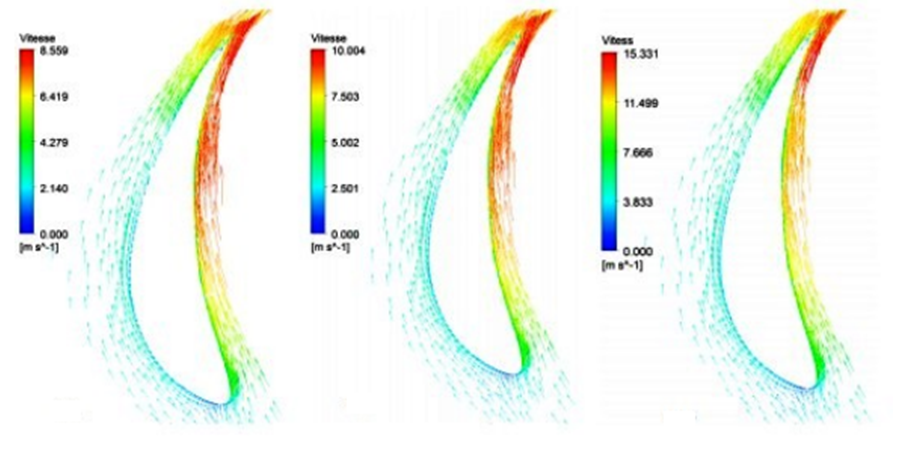 | Figure 6. Velocity field among the inlet guides (distributors) |
3.3. Velocity Profiles
The runner velocity generates the centrifugal forces which could affect many hydrodynamics parameters allowing the performance degradation of the Kaplan turbine. To well understand this phenomenon, we are going to describe the runner velocity influence on the axial and tangential velocities profiles at the entrance of the volute, compared to the experimental results of Behanu [8].The figures 7a & 7b below represent the axial velocity profiles at the entrance of the volute for different Reynolds numbers. The numerical and experimental results are in good concordance. We observe that the axial velocity is maxima at the downstream from the suction port of the Kaplan turbine.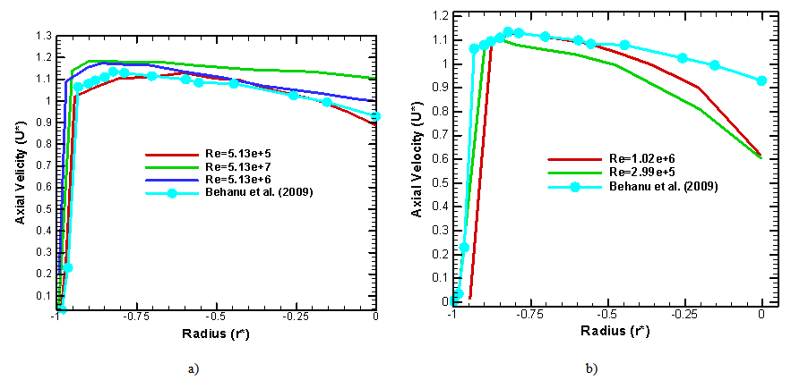 | Figure 7. Axial velocity profiles at the entrance of the volute; numerical and experimental [8] |
The figures 8a & 8b below represent the tangential velocity profiles at the entrance of the volute for different Reynolds numbers. The velocity profiles are periodic justifying the tangential movement generated by the runner rotation. We observe also the presence of a secondary flow. The experimental result of Behanu [8], are similar.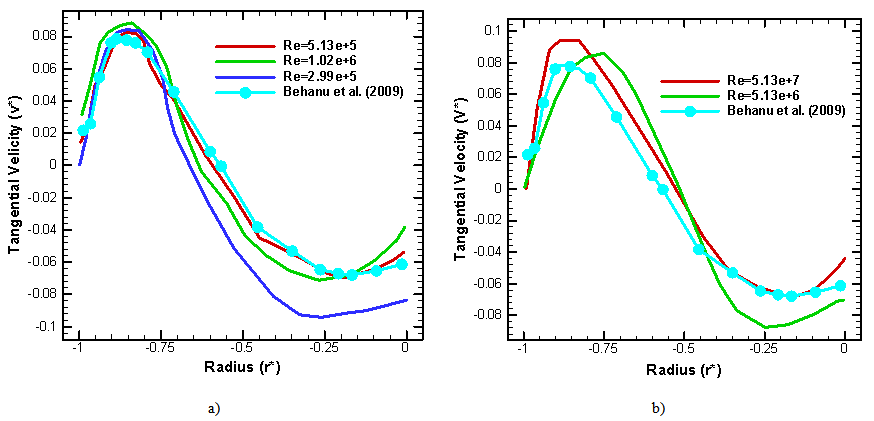 | Figure 8. Tangential velocity profiles at the entrance of the volute; numerical and experimental (Behanu [8]) |
3.4. Static Pressure Field
The figure 9 bellow represents the static pressure fields in the volute for different Reynolds numbers. We observe that the static pressure is high near the volute wall. This static pressure increases with the increasing of the Reynolds numbers up to the maximum value at the volute outlet. We observe also, for the high Reynolds numbers, a low of pressure around the volute medium. The pressure field is almost uniform and is characterized by a strong gradient of pressure inside the region near the outlet. The volute geometry generates a dissymmetry on the pressure field inside the turbine.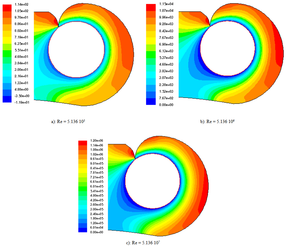 | Figure 9. Static pressure fields in the volute |
The figure 10 bellow represents the static pressure fields in the distributors. We observe that the static pressure is low at ring axis of the distributors. This value increases slowly up to distributor outlet. We observe also the formation of boundaries layers showing the gradual increasing of the axial velocity from the ring axis and a gradual decreasing of the tangential velocity.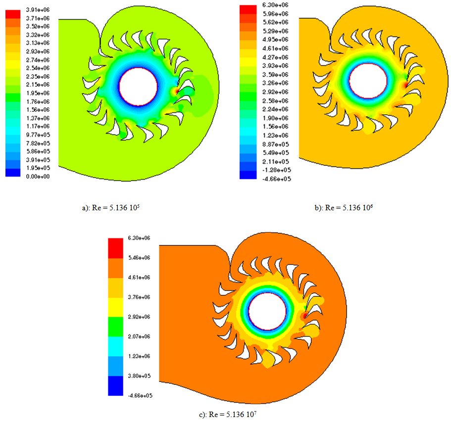 | Figure 10. Static pressure fields in the distributors |
4. Comparison of Results
The figures 11a & 11b bellow represent the axial velocity fields around the runner compared with the results of Behanu [8].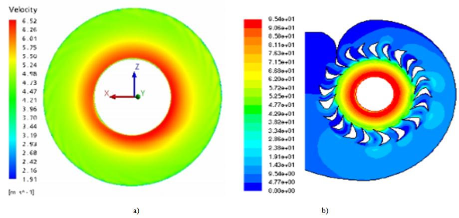 | Figure 11. Velocity fields around the runner for 595 rpm; a): Behanu [8], b): our results |
The figures 12a & 12b bellow represent respectively the experimental results obtained by LDA and PIV methods (Wu et al. [15]), and our numerical results. They show the static pressure field in the volute for a runner velocity of 596 rpm. The pressure increases gradually from the volute axis up to the wall. Our numerical results are similar.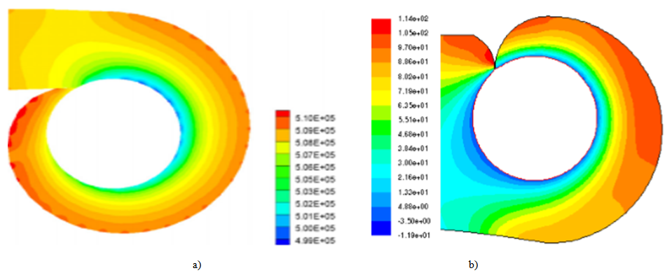 | Figure 12. Pressure fields in the volute for 595 rpm; a): Wu et al [15], b): our results |
The figures 13a & 13b represent the static pressure respectively of Wu et al. [15], and this present study, for the same runner velocity of 596 rpm. The experimental and numerical results are in good concordance.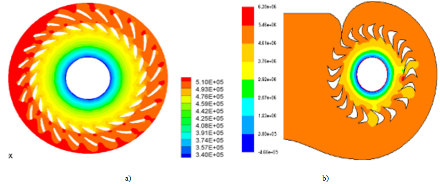 | Figure 13. Pressure fields in the distributor for 595 rpm; a): Wu et al [15], b): our results |
5. Conclusions
We have presented the pressure and velocity fields showing the separate zones and the zones of recirculation which influence the flow in the volute, distributors and around the runner of a Kaplan turbine. We have also presented the velocity profiles at the entrance of the Kaplan turbine volute. The comparison of our results with the experimental results of Behanu [8], and Wu et al. [15], shows a good agreement of the axial and tangential velocities. The static pressure is too high near the volute walls and inside the distributors. These qualitative considerations illustrated that the volute and distributors have an important rule on the Kaplan turbine performance.
Nomenclature
D: tube diameter (m)x: axial coordinate (m)y: vertical coordinate (m)L: draft tube length (m)v: vertical velocity (m/s)u: longitudinal velocity (m/s) mean of longitudinal velocity (m/s)
 Longitudinal velocity fluctuation (m/s)g: gravitational acceleration (m. s-2)P: pressure (N/m2)
Greek Symbols
ν: kinematic viscosity (m. Kg-1. s-1)ρ: density (kg. m-3)μ: dynamic viscosity (m. Kg-1. s-1)κ: turbulent kinetic energy (m3. s-2)ω: Specific dissipative rate (s-1) Krönecker symbol
 viscosity (m2/s)
 Shear stressΩ: vortexε: Deformation stress
References
| [1] | Duprat C., (2010). Simulation numérique instationnaire des écoulements turbulents dans les diffuseurs des turbines hydrauliques en vue de l’amélioration des performances. Thèse de Doctorat, Université de Grenoble, France. |
| [2] | Li WP, Li GX, Li H, and Zhang KW. (2008). Numerical simulation of water body resonance in penstock of hydropower station, Journal of Hydraulic Engineering, 39(1): 109–114. |
| [3] | Liu SH, Li SC, and Wu YL, (2009). Pressure fluctuation prediction of a model Kaplan turbine by unsteady turbulent flow simulation, ASME Journal of Fluids Engineering, 131(10): 101–112. |
| [4] | Petit O, Nilsson H, Vu T, Manole O, and Leonsson S., (2008). The flow in the U9 Kaplan turbine – preliminary and planned simulation using an open-foam. Proceedings of 24th IAHR symposium on hydraulic machinery and systems. Foz do Iguassu. |
| [5] | Zhou LJ, Wang ZW, Xiao RF, and Luo YY., (2007). Analysis of dynamic stresses in Kaplan turbine blades, Engineering Computational, 24(8): 753–762. |
| [6] | Merahi, M. Abidat, A. Azzi, and O. Hireche, (2002). Numerical assessment of incidence losses in an annular blade cascade. Séminaire Internationale de Génie Mécanique, Sigma’02 ENSET. Oran. 28 & 29 April Algeria. |
| [7] | L. Hilgenfeld, P. Stadtmuller, and L. Fottner, (2002). Experimental investigation of turbulence influence of wake passing on the boundary layer development of highly loaded turbine cascade blades. Unsteady flow in turbo machinery, V - 69, 3-4. Pp 229-247. |
| [8] | Behanu M. G., (2009). Experimental and Numerical Investigation of Axial Turbine Models, PhD. Thesis, Lulea University of Technology, Swede. |
| [9] | Launder B. E. and Spalding, D., (1974). The numerical computation of turbulent flow computational methods, Applied. Mechanical Engineering, Vol. 3, pp. 269-289. |
| [10] | Wilson D., (1998). Turbulence modeling for CFD. DCV industries, 2nd Edition. |
| [11] | Jones J. and Lauder B. E., (1961). A Single Formula for the Law of the Wall, Journal of Applied Mechanics, Vol. 28, No. 3: 444-458. |
| [12] | Patankar S.V., (1980). Numerical heat transfer and fluid flow, McGraw Hill, New-York. |
| [13] | Tcheukam-Toko, Mokem-Chetchueng M., Mouangué R., Beda T., Murzyn F., (2013). Characterization of Hydraulic Jump over an Obstacle in Open-channel Flow. International Journal of Hydraulic Engineering (IJHE), 2(5), 2013, 71-84. |
| [14] | Fluent (2006). User manual 6.3.26 |
| [15] | Wu Y., Shuhong D., Hua W., Shangfeng C., (2011). The numerical prediction and similarity study of pressure fluctuation in a prototype Kaplan turbine. Journal of Fluid Engineering. Vol. 15. |
 Abstract
 Reference
 Full-Text PDF
 Full-text HTML