G. G. Muscolo 1, S. Casadio 2, P. Forte 3
1Humanot s.r.l., Via Armando Spadini, 16, 50142, Firenze (FI), Italy
2GE Oil&Gas Headquarters, Nuovo Pignone S.p.A., via Felice Matteucci, 2 - 50127, Firenze (FI), Italy
3Dept. of Civil and Industrial Engineering, University of Pisa, Largo Lazzarino – 56122, Pisa (PI), Italy
Correspondence to: G. G. Muscolo , Humanot s.r.l., Via Armando Spadini, 16, 50142, Firenze (FI), Italy.
| Email: |  |
Copyright © 2012 Scientific & Academic Publishing. All Rights Reserved.
Abstract
In this paper the authors propose an innovative method for the determination of a transfer function (MTF) between the rotor responses on a balancing machine (HSB) and on turbo machinery (SP). The prediction of the rotor behavior in its turbo machine final housing is a crucial problem for turbo machinery manufacturers and very complex to solve using classical approaches. The proposed method uses a particular MTF formula, calculated with a black/box approach based on the application of the theory of System Identification, using the rotor responses in SP and in HSB as input and output respectively. MTF was determined by a regression analysis of the responses in HSB and SP of 10 rotors; subsequently it was tested and validated on other 15 rotors. The results demonstrate that proposed MTF simulates a rotor behavior in SP with a satisfactory overlapping of the measured output.
Keywords:
Rotor Dynamics, Balancing, System Identification, Vibrations, Black-Box, Transfer Function
Cite this paper:
G. G. Muscolo , S. Casadio , P. Forte , "Formulation of a Transfer Function between Rotor Responses on a High Speed Balancing Machine and in Turbo Machinery by System Identification", Energy and Power, Vol. 2 No. 6, 2012, pp. 107-115. doi: 10.5923/j.ep.20120206.01.
1. Introduction
The manufacturers of turbo machinery such as compressors, steam and gas turbines, usually construct the statoric parts and the rotor of the turbo machines in an independent way. Then assembly and test of the complete turbo machine take place before delivering the final product to the customer. The rotor is balanced several times on a high speed balancing machine (HSB) in order to reduce the gap error between the theoretical simulation and the real behavior of the rotor during the high speed rotation, thus it is positioned within the turbo machine (SP). The vibration limits of rotors and turbo machinery for proper operation are defined by ISO[1] and API[2].A very important problem, in the field of turbo machinery testing, is the prediction of rotor behaviour[3] in HSB and SP. Some rotors, with a stable behavior in rotation in theoretical simulation and balancing in HSB, have an unstable behavior during rotation tests in SP.In engineering problems, often the physical behavior of a system cannot be fully described (either for lack of baseline data or for excessive complexity of the system). In these cases it is necessary to use an experimental approach in order to define the mathematical model.System identification is utilized to solve this kind of problems[4]. The identification techniques generate a mathematical model using a regression analysis of the input or input-output data of a system[5, 6].In this paper the authors propose a new method based on a black-box approach to find a transfer function, called MTF[7], between the rotor responses on the High Speed Balancing machine (HSB) and in the turbo machine (SP). MTF allows to predict the vibration amplitude of the rotor in SP, already during the balancing steps in HSB. The black-box approach, proposed in this paper, was used because of the high complexity of the two systems and for the unavailability of all the data required to define accurate and realistic white-box models using classical approaches. This research was conducted in collaboration with a competitive Oil & Gas company and MTF represents a first relation between HSB and SP. The future planned steps are focused on the optimization of the formula (MTF) using a non-linear system identification approach. The paper is so structured: the first part presents the classical approaches used in order to solve the problem; the second part describes the proposed method and the third part reports MTF with the analysis and discussion of results.
2. Materials and Methods
The tests were carried out in the labs of GE Oil & Gas Company. In this study the rotors of compressors were considered because they have more problems in balancing (maybe related to impellers)compared to rotors of steam and gas turbines. In this study machines with horizontal rotor axis were used.
2.1. High Speed Balancing Machine (HSB)
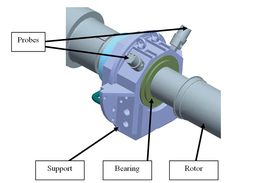 | Figure 1. Classical position of the two probes in a machine with horizontal rotor axis |
The vibration amplitude of the rotor is measured as function of the rotational speed[8, 9]. Inductive transducers (probes or non-contact sensors) are used to make these measurements. Usually, two probes are positioned on each bearing of the two supports of the HSB (Figure 1). The angular distance between the two transducers is 90° and they are positionedat 45° with respect to the vertical plane passing through the rotor axis for a balancing machine with horizontal rotor axis[10].A rotor is balanced if its vibration amplitude is lower than the threshold of 25 micrometers peak-to-peak in proximity of the first or second critical speed, as established by ISO and API[2, 3, 11]. Figure 2 shows a flowchart of a balancing process executed on the rotor of a compressor with two impellers.Many balancing steps are necessary before the final balancing test in HSB.
2.2. Turbo Machinery Testing (SP)
The turbo machinery test bench (SP) uses the same type of probes positioned in the same way with respect to the bearings of the rotor, as in HSB (Figure 1). The test performed in the turbo machinery lab is passed if the vibration amplitude of the rotor is below the threshold of 25 micrometers peak-to-peak in proximity of the first or second critical speed as in HSB[3]. If the test is not passed the rotor will be balanced again in HSB for several times and finally it will be tested again in SP.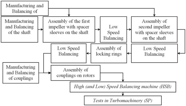 | Figure 2. Balancing process on the rotor of a compressor with two impellers |
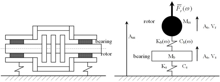 | Figure 3. Scheme of the rotor and of the models adopted for the fluid film bearing and for the support in the analytical studies |
3. Classical Approaches
3.1. Physical Approach
Figure 3 shows the scheme of a generic rotor and a simple 2 degrees of freedom model adopted to represent the fluid film bearings and the supports. Mb is the mass of the bearing and the support. Ks is the stiffness of the support and Kb is the stiffness of the fluid film of the bearing; Mrs is the mass of the rotor. Cb and Cs are the damping fluid film, respectively in the bearing and the support. Fr is the force of the rotor imbalance during rotation. Ar, Vr, As, Vs are amplitudes of vibration displacement (A) and velocity (V) respectively of the rotor relative to the bearing and of the bearing relative to the absolute system. Considering the vertical synchronous displacement, it is possible to correlate the vibration responses using probes (Ar) and velocimeters (Vs) by the following expression[12]: | (1) |
whereω is the angular speed of the rotor.ISO 11 342[13] defines a relationship between the maximum allowable speed of vibration of the rotor (or bearing) in the balancing machine (VHSB) and in the turbo machine (VSP), using three known proportional factors: | (2) |
Making the assumption that the supports in both testing conditions can be modelled in the same way, (1) and (2) allow to find the final relationship between the HSB and SP rotor responses: | (3) |
| Table 1. Differences between HSB and SP |
| | | SP | HSB | | Bearings | New | Recycled and used up to wear | | Oil temperature (TO):TO = constant = 60°C | Oil temperature (TO):TO ≈ 40°C | | Joint | Assembly at temperature T: T=25°C | Assembly at temperature T: T>25°C | | Vacuum | Notrigorous | Rigorous | | Runout (noise relative to probes[2],[11]) | 600-700 rpm. | 25% of the first critical speed (on average around 1000 rpm). |
|
|
Cd, Kd, Ct, Kt are damping (C) and stiffness (K) values in SP, respectively of the fluid film bearing (Cd, Kd,) and the support (Ct, Kt). Ar_HSB, andAr_SP are vibration amplitude values of the rotor respectively in HSB and SP. Md is the mass of the support and the bearing in SP.Equation (3) should help to determine theoretically a possible relationship between HSB and SP but, since it is based on simple linear models and not all the necessary input data are available, it can only provide qualitative information and cannot be used for an accurate prediction of the rotor behavior in SP.Table 1 lists some differences between HSB and SP that can generate different rotor behaviors.
3.2. Statistical Approach
A statistical analysis was also carried out considering 25 rotors. Table 2 shows the characteristics of the 25 rotors considered in the analysis. All of them respect the runout limit (runout is a noise relative to probes[2]) as defined in[11].| Table 2. Characteristics of the 25 analysed rotors |
| | Values | MAX | MIN | | Rotor masses(kg) | 1900 | 244 | | Diameter of impellers(mm) | 600 | 350 | | Number of impellers | 8 | 5 | | MCS = Maximum Continuous Speed (rpm) | 13027 | 8167 | | OS = Over Speed (rpm) | 14850 | 9310 | | TS = Trip Speed (rpm) | 13678 | 8657 |
|
|
Figure 4 shows vibration amplitudes of rotors number 9 and 12. One graph contains the vibration responses of four probes (A, B, C, D) in HSB overlapping to the four vibration responses in SP. A and B are the responses of the 2 probes mounted on the bearing of the support near to the motor transmission joint; C and D are the responses of the 2 probes mounted on the bearing on the other support.Many differences were noted among rotor vibration amplitudes in HSB and SP, especially near the first (3000-6000 rpm) or second (8000-12000) critical speed. A different behavior was also noted in nominally similar rotors (same dimensions and manufacturing process). The rotor number 9 (Figure 4) is similar in dimensions and manufacturing process to the rotor number 18 (Figure 5), but the vibration amplitudes of the two rotors are differentin HSB and SP.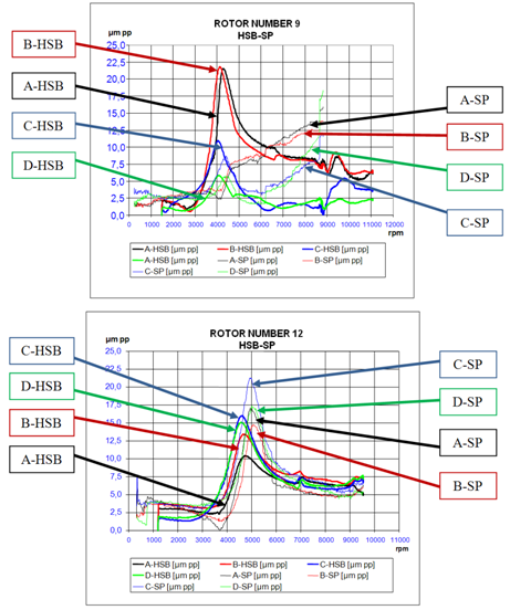 | Figure 4. Vibration Amplitude in micrometers peak-to-peak of rotors no. 9 and 12, in HSB and in SP. A, B, C, D represent the vibration responses measured by 4 probes on bearings in HSB e in SP |
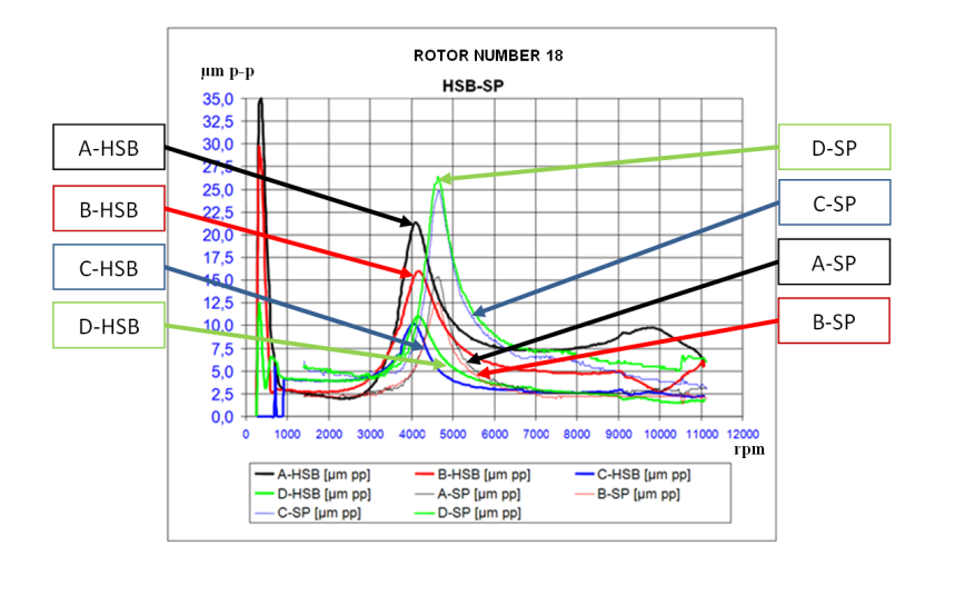 | Figure 5. Vibration Amplitude in micrometers peak-to-peak of rotors no.18 in HSB and in SP. A, B, C, D represent the vibration responses measured by 4 probes on bearings in HSB e in SP. The rotor no.18 is similar in dimensions and manufacturing process to the rotor no. 9 |
Figure 6 presents the scatter plots of rotor vibration amplitudes in SP (ordinate) and in HSB (abscissa) for 4 probes at different rpm. A poor correlation between rotor behavior in HSB and SP is observed.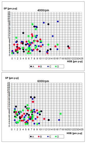 | Figure 6. Scatter plots of the vibration amplitude of 25 rotors in HSB (abscissa axis) and SP (ordinate axis). The graphs are reported at 4000 and 6000 rpm |
Tables 3 and 4 report the average vibration amplitudes of 25 rotors in HSB and SP respectively while Table 5 reports the mean and the standard deviation of the ratio of the vibration amplitude in HSB and SP of the 25 rotors. The standard deviation values are of the same order of magnitude of the mean values confirming a non-correlation between the amplitude values in HSB and SP.| Table 3. Mean and standard deviation of vibration amplitude values of 25 rotors in HSB |
| | HSB | PROBE | RPMx1000 | | 2 | 4 | 6 | 8 | 10 | 12 | | MEAN | A | 3.93 | 6.49 | 5.58 | 6.04 | 6.89 | 7.42 | | B | 3.86 | 6.68 | 5.66 | 5.99 | 5.79 | 8.22 | | C | 4.35 | 8.13 | 6.00 | 7.02 | 8.39 | 10.86 | | D | 3.89 | 6.72 | 5.64 | 5.97 | 7.38 | 6.31 | | STANDARD DEVIATION | A | 2.67 | 4.82 | 3.22 | 3.69 | 5.02 | 4.82 | | B | 2.27 | 4.81 | 2.63 | 3.36 | 5.14 | 5.39 | | C | 3.09 | 4.31 | 3.65 | 4.33 | 5.78 | 4.38 | | D | 3.00 | 3.4 | 3.56 | 4.19 | 3.81 | 3.96 |
|
|
| Table 4. Mean and standard deviation of vibration amplitude values of 25 rotors in SP |
| | SP | PROBE | RPMx1000 | | 2 | 4 | 6 | 8 | 10 | 12 | | MEAN | A | 2.85 | 6.58 | 7.05 | 7.56 | 5.27 | 6.41 | | B | 2.92 | 5.48 | 6.5 | 6.32 | 5.3 | 6.35 | | C | 3.73 | 7.14 | 5.42 | 5.08 | 4.87 | 6.39 | | D | 3.72 | 6.28 | 5.83 | 5.34 | 4.85 | 6.15 | | STANDARD DEVIATION | A | 2.00 | 4.87 | 3.94 | 6.64 | 3.73 | 5.36 | | B | 1.95 | 2.80 | 3.34 | 4.65 | 3.60 | 5.15 | | C | 2.62 | 5.02 | 3.65 | 2.85 | 2.86 | 4.35 | | D | 2.59 | 4.35 | 3.23 | 3.04 | 2.51 | 3.28 |
|
|
| Table 5. Mean and standard deviation of the ratio (HSB-SP) of the vibration amplitude values of 25 rotors |
| | HSB/SP | PROBE | RPMx1000 | | 2 | 4 | 6 | 8 | 12 | | MEAN | A | 2.06 | 1.44 | 1.01 | 1.21 | 1.63 | | B | 1.93 | 1.77 | 1.05 | 1.30 | 1.71 | | C | 1.91 | 1.57 | 2.02 | 1.82 | 1.91 | | D | 1.58 | 1.60 | 1.57 | 1.74 | 1.22 | | STANDARD DEVIATION | A | 2.65 | 1.49 | 0.93 | 1.01 | 2.39 | | B | 2.35 | 2.57 | 0.74 | 1.17 | 2.50 | | C | 2.52 | 1.58 | 2.43 | 1.80 | 2.48 | | D | 1.88 | 1.51 | 2.05 | 2.15 | 1.30 |
|
|
Figure 7 shows the average vibration amplitudes of 25 rotors in HSB and SP. A shift can be noted in the amplitude values at the first and second critical speeds in SP with respect to HSB towards higher and lower rpm respectively. This is probably due to the influence of the transmission joint and of the bearings that are different in HSB and SP (Table 1).In conclusion the results of the statistical approach suggest a non-linear and more complex nature of the relationship between the two responses.
4. LinearSystemIdentification: Black-Box Approach
Statistical and physical approaches have highlighted the difficulties of representing the complex relation between the HSB and SP systems and the need to use other tools to identify such a relation.The new method proposed in this article allows determining the transfer function between HSB and SP for rotors with the characteristics listed in Table 2, within the range of rotational speed from 1000 rpm to 12000 rpm.A black-box approach, based on the theory of system identification[5, 6], was utilized in order to determine the transfer function. In the proposed method, the rotor responses in HSB and SP were considered, respectively, as an input (H) and output (S) signal; a mathematical model using a regression analysis of input-output data of the system H-S was created. The transfer function linking these two signals (H and S), for each single rotor, was a particular solution. The general formula, valid for all rotors, relating H and S (and then HSB and SP), called MTF[7], was constructed from the subsequent analysis of many particular solutions.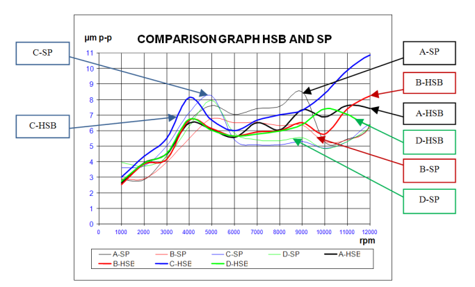 | Figure 7. Comparison between average values in HSB and SP |
4.1. Analysis and Processing of Experimental Data
25 different rotors by weight, length, number of impellers, etc. (see Table 2) were considered for the determination and validation of MTF.For the sake of simplicity, instead of the rotational speed in rpm, the following variable was adopted: | (4) |
For each rotor it is possible to get two signals, H and S (as input and output), for each probe (A, B, C, D), expressed as a function of variable i ranging from 0 to 110 corresponding to a range of rotational speed from 1000 to 12000 rpm.The signal was sampled from 1000 rpm (0i) to 12000 rpm (110i) (period Ti = 110), with spaces of variable Δi = 1, satisfying the sampling theorem (Shannon theorem). Eight data vectors[111x1] were created for each rotor, corresponding to the eight signals of the probes (figure 4). Four input data vectors (in HSB (H)) and four output data vectors (in SP (S)) were considered. Each vector is formed by a column of values and by 111 lines of sampling. The signal analysis[1] was carried out on the data vectors[111x1]. The process of analysis of 10 rotors is described in the following sections with reference to probe A; for the other probes the procedure is the same. 10 input and 10 output vectors were constructed; three systems of data were built: one system was obtained without data filtering, one was obtained with constant detrend (removing mean value) and another system was obtained using linear detrend.
4.2. Identification Process, Optimal Model and Its Validation
The first step of identification techniques is understanding what family models can describe the data. The analysis was limited to five linear family models: ARX, ARMAX, OE, BJ, PEM[5]. The second step of identification techniques is the determination of the complexity of the model by varying its order. In this paper the Final Prediction Error (FPE) and the Akaike Information Criterion (AIC) were used as prediction error[4, 5]. The optimal order of a model corresponds to the lowest calculated values of AIC and FPE[5]. Each rotor was analysed using Matlab System Identification Toolbox and the validation was done using Simulink.In order to determine the transfer function, tests and simulations were performed on 10 rotors using parametric models (arx, armax, oe, bj) and models for signal processing (or prediction error (PEM)), with different polynomial order. For both models (parametric and pem) 3 types of analysis of values were carried out: without detrend, with average detrend (order 0) and with linear detrend (order 1).The comparison of all models and the subsequent simulation allowed to choose model bj22221. Among all families the bj model best describes, with the lowest percentage error, the sequence of data of H and S (HSB and SP) for all 10 rotors. The bj22221 model, among the stable models, has the lowest values of AIC and FPE[5], respectively equal to 0.0963 and 2.3401.
5. Transfer Function (MTF) between HSB and SP
5.1. MTF
MTF is the proposed transfer function between HSB and SP defined by the determination of coefficients, α(q), β(q), γ(q) and δ(q), of model bj22221: | (5) |
where: ;
; ;
; ;
; ;The elements of vectors H(i) and S(i) are the vibration amplitude values of 4 probes respectively obtained in HSB and SP varying the value of the variable i (
 ). Equation (5) is based on a BJ family model[5] and with MTF it is possible to obtain the simulation of vibration amplitude values of the rotor in the turbo machinery bench SP (S(i)), giving vector H(i) as input.In conclusion, by using MTF it is possible to obtain the simulation of the trend of vibration amplitudes in SP knowing the vibration amplitude values in HSB at the end of the rotor high speed balancing.
5.2. Results and Discussion
MTF was determined by analysing the trends of 10 rotors (rotor no.1 to 10) and it was validated on other 15 different rotors (rotor no.11 to 25).The following figures show measured, simulated and predicted output graphs. The figures reproduce the real (S) andpredicted output signal (MTF) using only input data history (H).The right side of the plot, in the figures, displays the percentage of the output that MTF reproduces (Best Fit), computed using the following equation: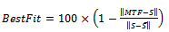 | (6) |
MTFis the simulated or predicted model output, S is the measured output and  is the mean of S. 100% corresponds to a perfect fit, and 0% indicates that the fit is no better than guessing the output to be a constant
  .Figure 8 shows real (S) and simulated (MTF) responses respectively of three rotors. Not all the trends of the 10 rotors, used to determine MTF, have the same fit, but in all rotors the signal simulated with MTF follows the real one for its entire length.From the graphs of the following figure it is also possible to note the difference of rotor behavior in SP: rotor no.2 (S2 in Figure 8) has a maximum limit of 10 micrometers peak-to-peak at the first critical speed
  and has a value lower than 25 micrometers peak-to-peak at the second critical speed (
 ); for rotor no.6 (S6 in Figure 8) the first critical speed has a value of 18 micrometers peak-to-peak
  and the second critical speed has a value lower than 6 micrometers peak-to-peak (
 ). The other rotors have different responses indicating the non-linearity of the system.Figure 8 shows the values of best fit in simulation equal to 26.9%, 47.8% and 43.3% respectively for graphs S2, S5 and S6. The other rotors have best fit values in simulation that range from 15% to 44.2% with the exception of one rotor that got a negative value because the estimation algorithm failed to converge using linear system identification. Such a result means that it is necessary to try non linear identification. Moreover the obtained graphs show that the formula needs to be optimized.Except for six rotors that got negative predicted values the predicted MTF responses of the rotors of the validation group confirm that MTF reproduces satisfactorily the experimental response with best fits that range from 22.5% to 57.5%.
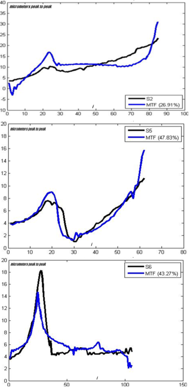 | Figure 8. Determination of MTF: measured (S2, S5, S6) and simulated model output (MTF) of rotors no.2, 5 and 6 |
Figure 9 shows the measured and predicted model output using MTF for three of the rotors used for validation, no. 13, 15and 22. Using the best fit definition of equation (6) the fit values obtained for these rotors are respectively: 36.1% for rotor no. 13 (S13), 57.5% for rotor no. 15 (S15), 32.9% for rotor no. 22 (S22).In some cases the predicted response generates a trend similar to the real signal, but for shifts in frequency of the critical speeds. However, in all cases, the order of magnitude of the peak amplitudes of the predicted response is the same of the real one and that can already be a useful indication.Best fits in the range of 15% - 48% for 10 rotors and in the range of 22.5% - 57.5% for 15 rotors are good results for rotors like those considered in table 2. Actually, using classical approaches the range of best fits is wider.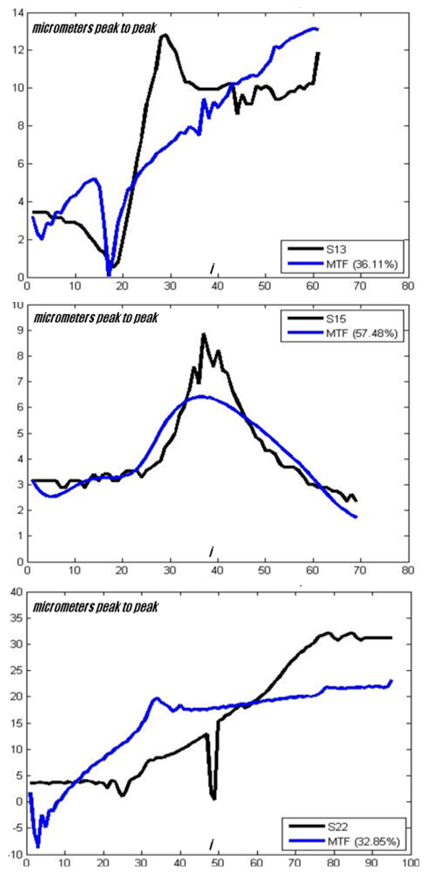 | Figure 9. Validation of MTF: measured (S13, S15, S22) and predicted output (MTF) of rotors no. 13, 15 and 22 |
The validation of MTF was also confirmed in the prediction of the trends of the other 3 remaining probes (B, C and D), corresponding to the other six lines of the graphs of Figure 4 analysed in addition to probe A considered in this article.Validation of MTF for the three probes gave the following results. Probe B, for all 25 rotors has the same trends of probe A, at least near the first critical speed. In proximity to the second critical speed it seems that probe B reproduces, in some cases, responses similar to probe C. The trends of probe C are predicted with the same goodness of probe A. For most of the rotors probe D has the same trends in prediction of probe C. For some rotors, near the second critical speed, probe D follows probe A, whereas probe B follows probe C.The transfer function MTF is representative for the probe that has the largest number of resonances (probe A).
6. Conclusions and Future Works
In this paper the authors, having considered the limitations of the classical (physical and statistical) approaches, the high complexity of the systems and the unavailability of the necessary data, used a black-box approach based on system identification to find a transfer function, called MTF[7], between the rotor responses on a high speed balancing machine (HSB) and in turbo machinery (SP).MTF was determined by a regression analysis of the responses in HSB and SP of 10 rotors; subsequently it was tested and validated on other 15 rotors.The tests were carried out in the labs of GE Oil & Gas Company. Only the rotors of compressors were considered because they have more problems in balancing (maybe related to impellers) compared to rotors of steam and gas turbines. This research started because some of these rotors presented a stable response in HSB and an unacceptable response in SP. The results of this paper demonstrate that MTF simulates a rotor behavior in SP with a satisfactory overlapping of the measured output. MTF should allow to predict the vibration amplitude of the rotor in SP, already during the balancing steps in HSB. The proposed formula is the first attempt to find a relation between the two systems (HSB and SP) and must be considered preliminary. The linear system identification models, studied in this paper, are actually a first step of this research. In fact the best fit negative value obtained for some rotors indicate that the estimation algorithm failed to converge using linear identification and that it is necessary to apply non-linear identification methods. Moreover, the formula was obtained on the basis of the signals of one probe but with some additional work it could be optimized on the responses of all the other probes. Improvements could be made also differentiating the formula for classes of rotors or for ranges of operating conditions.The future planned steps are therefore focused on the optimization of the formula using a non-linear system identification approach.
ACKNOWLEDGMENTS
The authors acknowledge the support of GE Oil&Gas Company.
References
| [1] | ISO 7475-2002 “Mechanical vibration – Balancing machines – Enclosures and other protective measures for the measuring station”, International Organization of Standardization. |
| [2] | American Petroleum Institute, “Tutorial on the API Standard Paragraphs Covering Rotor Dynamics and Balancing: An Introduction to Lateral Critical and Train Torsional Analysis and Rotor Balancing“, API Publication 684 (p. 117) (Washington, D. C.: American Petroleum Institute, 1996). |
| [3] | M.S.Darlow, “Balancing of High-Speed Machinery”,Springer-Verlag, 1989. |
| [4] | LennartLjung, “System Identification: Theory for the user”, 2nd ed., PTR Prentice Hall, Upper Saddle River, N. J. – 1999. |
| [5] | H. G. Natke, “Application of system identification in engineering”, CISM courses and lectures No. 296. International centre for mechanical sciences; Springer Verlag Wien – New York (pp.198 – 231) 1988. |
| [6] | Draper N. R. and Smith H., “Applied regression analysis”, New York John Wiley and Sons. |
| [7] | G. G. Muscolo, “Determinazione di unafunzione di trasferimentotral’impianto di equilibraturarotori e la sala test finale della GE Oil&Gas”, Master’s Thesis, Department of Mechanical, Nuclear and Manufacturing Engineering, University of Pisa - Italy, December 2008 (In Italian. English Abstract). |
| [8] | Fredric F. Ehrich, “Handbook of Rotordynamics“, McGraw - Hill – 1992. |
| [9] | D. E. Bently, C. T. Hatch, B. Grissom, “Fundamentals of rotating machinery diagnostics“, chapter 13 ( pp. 249 – 272 ), 16 (pp. 337-382) and 23 (pp. 499-515), 2002. |
| [10] | American Petroleum Institute, “Axial and Centrifugal Compressors and Expander-Compressors for Petroleum, Chemical and Gas Industry Services”, API standard 617 (Washington, D. C.: American Petroleum Institute, 1996). |
| [11] | S. Timoshenko, W. Weaver, Donovan H. Young, “Vibration problems in engineering”, John Wiley & Sons inc. V edition, 1990. |
| [12] | ISO 1940/2-1997 “Mechanical Vibration - Balance quality requirements of rigid rotors - Part 2: Balance errors”, International Organization of Standardization. |
 Abstract
 Reference
 Full-Text PDF
 Full-Text HTML