1. Introduction

Small signal stability analysis of power systems has become more important nowadays. Under small perturbations, this analysis predicts the low frequency electromechanical oscillations resulting from poorly damped rotor oscillations. The oscillations stability has become a very important issue as reported in [4-6]. The operating conditions of the power system are changed with time due to the dynamic nature, so it is needed to track the system stability on-line. To track the system, some stability indicators will be estimated from given data and these indicators will be updated as new data are received. Synchronising torque coefficients, K_s and damping torque coefficients, K_d are used as stability indicators. To achieve stable condition, both the K_s and K_d must be positive [1-3].

Certain techniques have been proposed to estimate the values of K_s and K_d involving optimisation technique. Some techniques have been explored by means of frequency response analysis [6,7]. [3] decomposed the change in electromagnetic torque into two orthogonal components in the frequency domain. The two equations were expressed in terms of the load angle deviation then solved directly. Static and dynamic time domain estimation methods were also proposed in this study.

Least Square (LS) method can be one of the possibletechniques in addressing the stable and unstable phenomena. It has been used as static parameter estimation [8]. However, several disadvantages have been identified in LS method. Amongst them are the long computation time and the requirement for data updating. It also requires monitoring the entire period of oscillation.

Recently, optimisation algorithms such as Evolutionary Programming (EP) and Artificial Intelligent System (AIS) have received much attention in global optimisation problems. EP and AIS are heuristic population-based search methods that use both random variation and selection. The optimal solution search process is based on the natural process of biological evolution and is accomplished in a parallel method in the parameter search space. EP-based method has been applied in various researches in static [12-16] and dynamic system stability [17-19]. On the other hand, AIS optimisation approach is still new in power system compared to the EP. EP and AIS share many common aspects; EP tries to model the natural evolution while AIS tries to benefit from the characteristics of human immune system [20-22].

This paper presents an efficient online estimation technique of synchronising and damping torque coefficients in solving angle stability problems. It is based upon the population-based search methods that use both random variation and selection. The method is used to estimate synchronising torque coefficients, K_s, and damping torque coefficients, K_d, from the machine time responses of the change in rotor angle, Δδ(t), the change in rotor speed, Δω(t), and the change in electromechanical torque, ΔT_e(t). The goal is to minimise the estimated coefficient error and the time consumed. The proposed EP technique is used to find the best solution of the formulated problem. Results obtained from the experiment using EP were compared with AIS and LS methods. Then, the results were verified with eigenvalues.

2. The System Model

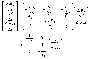
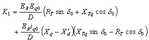
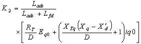
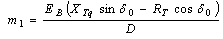
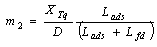
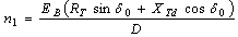
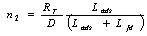
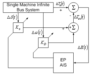
A simplified block diagram model of the small signal performance is shown in Figure 1. In this representation, the dynamic characteristics of the system are expressed in terms of K constants with linearised single machine infinite bus (SMIB) system. This model is represented with some variables such as electrical torque, rotor speed, rotor angle, and exciter output voltage.

Figure 1. Block diagram model of small signal performance.

As in the case of the classical generator model, the acceleration and the field circuit dynamic equations are:

(1)

(2)

(3)

where T_m is a mechanical torque, T_e is a electromagnetic torque, e_fd is a field voltage, R_fd is a rotor circuit resistance, i_fd is a field circuit current, and ω₀=2πf₀.

From the transfer function block diagram, the following state-space form is developed.

(4)

The system matrix A is a function of the system parameters that depends on the opening conditions. The perturbation matrix B depends on the system parameters only. The interaction among these variables is expressed in terms of the 4 constants K₁, K₂, K₃, and K₄. Constants K₁, K₂, and K₄ are functions of the operating real and reactive loading as well as the excitation levels in the generator. K₃ is a function of the ratio of impedance. Details of matrix A and matrix B are explained as follows.

(5)

(6)

(7)

(8)

(9)

(10)

(11)

(12)

(13)

(14)

(15)

(16)

(17)

(18)

(19)

(20)

(21)

(22)

(23)

(24)

(25)

(26)

(27)

P_t and Q_t are terminal active and reactive power, respectively. All related equations are given in [1].

3. The System Model

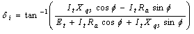
A single machine connected to infinite bus system is considered. The system comprises a steam generator connected via a tie line to a large system represented as infinite bus. The machine differential equations, the exciter equation, and the block diagram can be found in [1].

The change of electromagnetic torque ΔT_e(t) can be broken down into two components namely the synchronising torque, K_s and damping torque, K_d. The synchronising torque is in phase and proportional with the change in rotor angle, Δδ(t), while the damping torque is in phase and proportional with the change in rotor speed, Δω(t). The estimated torque, ΔT_es(t) can be written as:

(28)

where:

Δδ(t): Change in rotor angle

Δω(t): Change in rotor speed

K_s: Synchronising torque coefficients

K_d: Damping torque coefficients

4. Evolutionary Programming

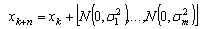
The Evolutionary Programming (EP) is one of the evolutionary computing techniques that uses the models of biological evolutionary process to solve complex engineering problems. The search for an optimal solution is based on the natural process of biological evolution and is accomplished in a parallel method in the parameter search space. EP belongs to the generic fields of simulated evolution and artificial life. It is robust, flexible, and adaptable and it can yield global solutions to any problem, regardless of the form of the objective function.

The advantages of EP over other conventional optimisation techniques can be summarised as follows [12-19]:

(a) EP searches the problem space using a population of trials representing possible solutions to the problem and not a single point. This will ensure that EP has less possibility of getting trapped in local minima. Therefore, EP can reach to a global optimal solution.

(b) EP uses performance index or objective function information to guide the search for solution. Therefore, EP can easily deal with non-smooth and non-continuous objective functions.

(c) EP uses probabilistic transition rules instead of non-deterministic rules to make decisions. Moreover, EP is a kind of stochastic optimisation algorithm that can search a complicated and uncertain area to find the global minimum. This makes EP more flexible and robust than conventional methods.

In the EP algorithm, the population has 2n candidate solutions with each candidate solution is an m-dimensional vector, where m is the number of optimised parameters. The EP algorithm can be described as:

• Step 1 (Initialisation): Generation counter i is set to 0. n random solutions (x_k, k=1, …, n) are generated. The k^th trial solution x_k can be written as x_k=[p₁ ,…, p_m], where the l^th optimised parameter p_i is generated by random value in the range of [p_l^min, p_l^max] with uniform probability. Each individual is evaluated using the fitness J. In this initial population, minimum value of fitness, J_min will be searched; the target is to find the best solution, x_best with the fitness, J_best.

• Step 2 (Mutation): Each parent x_k produces one offspring x_k+n. Each optimised parameter p_l is perturbed by Gaussian random variable N (0, σ_l²). The standard deviation, σ_l specifies the range of the optimised parameter perturbation in the offspring. σ_l can be written as follows:

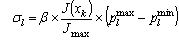(29)

where β is a search factor, and J(x_k) is the fitness equation of the trial solution, x_k. The value of optimised parameter will be set at certain limit if any value violates its specified range. The offspring x_k+n can be described as:

(30)

where k=1, …, n

• Step 3 (Statistics): The minimum fitness, J_min; the maximum fitness, J_max; and the average fitness, J_ave of all individuals are calculated.

• Step 4 (Update the best solution): If J_min is bigger than J_best, go to Step 5, or else, update the best solution, x_best. Set J_min as J_best, and go to Step 5.

• Step 5 (Combination): All members in the population x_k are combined with all members from the offspring x_k+n to become 2n candidates. Matrix size would be [2n × k] from its original size [n × k], where k is the number of control variables. These individuals are then ranked in descending order based on their fitness as their weight.

• Step 6 (Selection): The first n individuals with higher weights are selected as candidates for the next generation.

• Step 7 (Stopping criteria): The search process will be terminated if one of the followings is satisfied:

i It reaches the maximum number of generations.

ii The value of (J_max − J_min) is very close to 0.

If the process is not terminated, the iteration process will start again from Step 2. The flowchart of EP is shown in Figure 2.

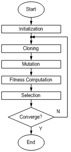
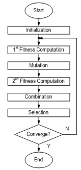Figure 2. Flowchart of EP

5. Artificial Immune System

Artificial immune system (AIS) approach to optimisation is more recent exploitation of natural phenomena in power system than EP. EP and AIS share many common aspects. Unlike the EP that tries to model the natural evolution, AIS tries to benefit from the characteristics of human immune system. Basic algorithm for AIS-based optimisation is called the Clonal Selection Algorithm (CSA) and it works as follows [20-22]:

• Step 1: Initialisation; during initialisation, n random solutions (xk, k=1, …, n) are generated to represent the control parameters and determine the fitness, J.

• Step 2: Cloning; population of variable x will be cloned by 10. As a result, the number of cloned population becomes 10n. Each individual of cloned population is evaluated using the J. Minimum value of fitness, Jmin will be searched; the target is to find the best solution, xbest with the best fitness, Jbest.

• Step 3: Mutation; each individual clone is mutated. The mutation equation can be described as in equation (30) and (31).

• Step 4: Ranking process; the population of matured clones in Step 2 and mutated clones in Step 3 are ranked based on fitness. The first n individuals with higher weights are selected along with their fitness as parents of the next generation.

• Step 5: Convergence test; The search process will be terminated if one of the followings is satisfied:

i It reaches the maximum number of generations.

ii The value of (Jmax − Jmin) is very close to 0.

If the process is not terminated, the iteration will repeat from Step 2 again. The flowchart of AIS is shown in Fig. 3.

Figure 3. Flowchart of AIS

6. Least Square Method

All the data of Δδ(t), Δω(t), and ΔT_e(t) can be obtained from either offline simulation or online measurements. Following a small disturbance, the time responses of these three items are recorded. The least square (LS) method is then used to minimise the sum of the square of the differences between the electric torque, ΔT_e(t) and the estimated torque, ΔT_es(t). The error is defined as:

(31)

The torque coefficients, K_s and K_d are calculated to minimise the sum of the error squared over the interval of oscillation, t as given in equation (4), where t=NT (N is the number of samples and T is the sampling period). For correct estimation of K_s and K_d, the interval t should be chosen adequately. The suitable value of t that makes K_s and K_d constant during the oscillation period was found to be the entire period of oscillation. In matrix notation, the above problem can be described by an over-determined system of linear equations as follows:

(32)

where A=[Δδ(t) Δω(t)], and x=[K_s K_d]^T. The estimated vector, x is such that the function J(x) is minimised, where:

(33)

In this case, the estimated vector, x will be given by:

(34)

where A^t is the left pseudoinverse matrix. Solving equation (35) gives the values of K_s and K_d for the corresponding operating point.

7. Test System

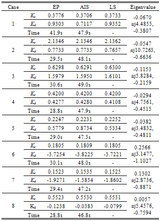
In this study, performance evaluation of the EP for the estimation of K_s and K_d is compared with LS and AIS estimation methods. The evaluation is carried out by conducting several offline simulation cases on the linearised model of SIMB. In this study, block diagram as shown in Figure 1 is used for offline simulation to generate the required Δδ(t), Δω(t), and ΔT_e(t) samples in MATLAB Simulink environment.

Figure 4. Estimating Ks and Kd using EP and AIS

Table 1. Eight different loading conditions.

The SMIB system parameters are as follows:

Generator parameters:

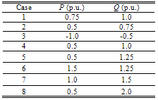
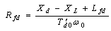
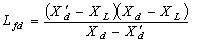
H = 2.0, T_d0^’ = 8.0, X_d = 1.81, X_q = 1.76, X_d^’ = 0.30, R_a = 0.003, K_sd = K_sq = 0.8491, E_t = 1.0−36°

Transmission line parameters:

R_e = 0.0, X_e = 0.65, X_L = 0.16

where T_d0^’ is the open circuit field time constant; X_d and X_q are the d-axis and q-axis reactance of the generator, respectively; R_a and X_d^’ are the armature resistance and transient reactance of the generator, respectively; R_e and X_e are the resistance and reactance of the transmission line, respectively; X_L is the load reactance; K_sd and K_sq are the d-axis and q-axis of synchronising torque coefficients, respectively; and E_t is the terminal voltage.

Stable and unstable study cases are simulated using different types of disturbances. Data size is set to 20 seconds, while number of samples is set to 400 samples. Using Δδ(t), Δω(t), and ΔT_e(t) as generated sample data, 2 sets of MATLAB files, EP and AIS-based simulation are developed. The simulation diagram is shown in Figure 4.

In this study, eight sets of of Δδ(t), Δω(t), and ΔT_e(t) samples are generated using offline simulation implemented in MATLAB Simulink. Those eight different loading conditions are tabulated in Table 1.

During simulation, all parameters are adjusted until an optimal solution is obtained. The results of EP and AIS are compared with the LS solution.

8. Simulation Results

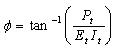
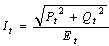
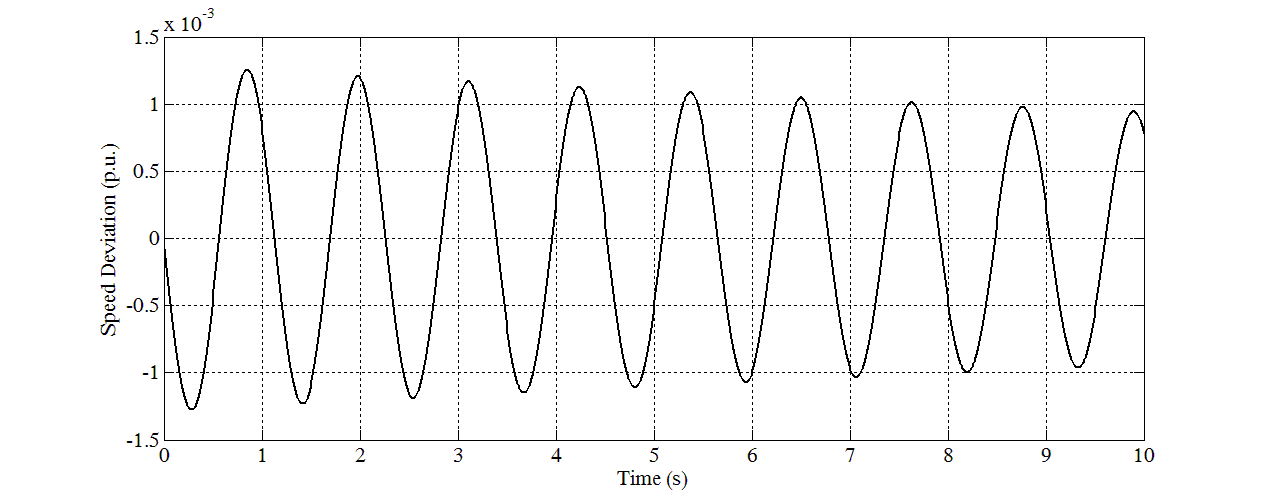
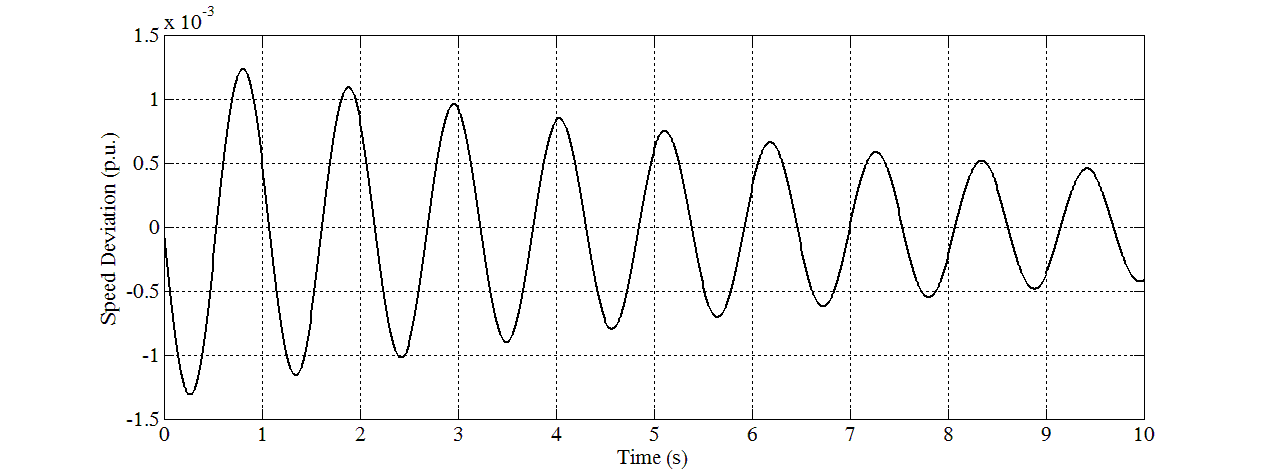
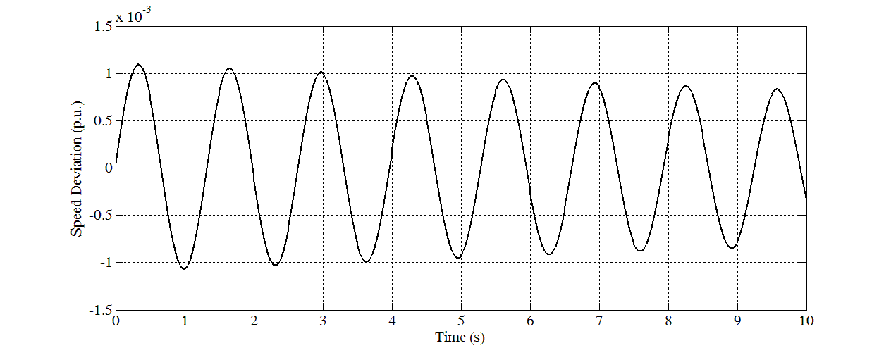
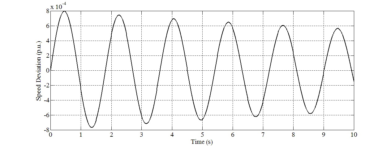
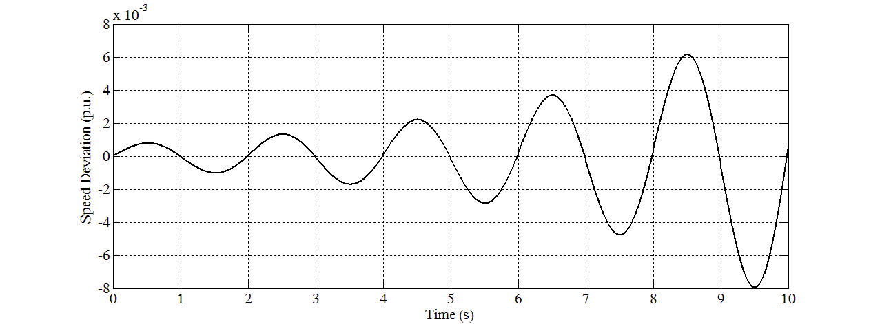
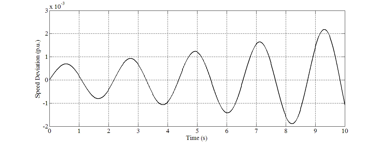
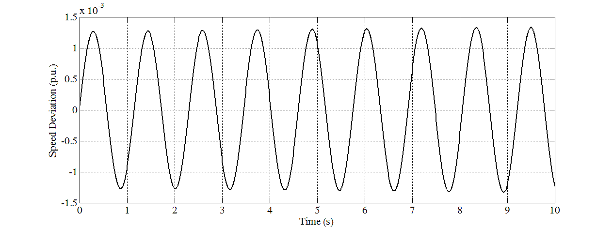
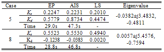
In this study, eight sets of Δδ(t), Δω(t), and ΔT_e(t) samples are generated using offline simulation of block diagram implemented in MATLAB Simulink. The samples of Δδ(t) data in graph forms are shown in Figure 5 until Figure 12. Different values of P and Q are used to simulate these cases. For verification, the eigenvalues for all cases have been calculated and written below of each graph. For cases in which all the eigenvalues are negative, they are stable. For cases that have positive eigenvalues, they are unstable.

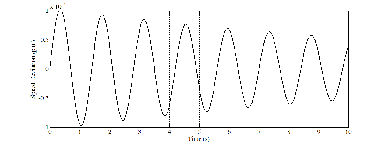Figure 5. Speed response for Case 1

Figure 6. Speed response for Case 2

Figure 7. Speed response for Case 3

Figure 8. Speed response for Case 4

Figure 9. Speed response for Case 5

Figure 10. Speed response for Case 6

Figure 11. Speed response for Case 7

Figure 12. Speed response for Case 8

Table 2 shows the results obtained from the eight study cases. The estimated constants obtained using EP, AIS, and LS methods are shown as well as the eigenvalues for each case.

From the results of eigenvalues, the first five cases (Figure 5 until Figure 9) are stable and the other three cases (Figure 10 until Figure 12) are unstable. As both values of K_s and K_d are positive, the results indicate that case 1, 2, 3, 4, and 5 are stable cases. On the other hand, case 6, 7, and 8 are unstable cases as the value of K_d is negative. Eigenvalues shown in the last column verify the results obtained.

In all cases, all three methods give accurate and close results. Although results using EP and AIS methods are close, the difference in the value between EP and LS methods is closer than the difference in the value between AIS method and LS methods. This shows that simulation results from EP method are more accurate and closer than simulation results using AIS method.

Except for LS method, the time consumed to calculate the values of K_s and K_d until they reach steady state solution has been recorded for EP and AIS methods. As the calculated values of K_s and K_d are same with the first iteration, the time consumed for LS method is not recorded. Comparing the EP and AIS for all cases, the average of time consumed to calculate using AIS is about 48 seconds, while the average of time consumed to calculate using EP is about 30 seconds. This shows that the average of time consumed to calculate using AIS is almost 40% longer than using EP. This also means that calculation method using EP is faster than AIS.

For the effect of error-contaminated data on the accuracy of the estimated values of K_s and K_d, simulation is done by introducing about 10% of bad data (zeros) at different locations of Δδ(t), Δω(t), and ΔT_e(t). For comparison, case 5 and 8 are selected.

Table 2. Results of EP, AIS, LS, and eigenvalues for case 1 until 8

Table 3 shows the results of EP, AIS, and LS methods calculation with bad data. It is clear that although bad data are injected into the system, estimates for K_s and K_d using EP and AIS methods are not affected as the value is identical with the results obtained in Table 2.

On the other hand, LS method is affected with the 10% of bad data introduced. Moreover, it also gives false result for case 8. Using the LS method, the simulation gives positive value of damping torque coefficient, K_d, which indicates that the system is stable for case 8. But, the results given by EP and AIS methods give negative value, which indicates that the system for case 8 is unstable. This result can also be confirmed by the positive value of eigenvalues, which verifies that case 8 is unstable. As a result, estimates for K_s and K_d using EP and AIS method are more accurate compared to LS method.

Table 3. Results of EP, AIS, LS, and eigenvalues for case 5 and case 8 with bad data.

9. Conclusions

In this paper, three methods for accurate estimation of the synchronising and damping torque coefficients, K_s and K_d are presented. The performance of Evolutionary Programming (EP) is compared with the Artificial Immune System (AIS) and Least Square (LS) methods. In comparison with AIS and LS methods, EP offers several advantages. These include better data accuracy and 60% shorter computing time compared to AIS. EP is also not affected with bad data consumed in the system unlike the LS method that gives false decision on the stability. The proposed method can be considered a reliable and efficient tool in the area of power system stability analysis.