A. Thabet1, M. Boutayeb2, G. Didier3, S. Chniba4, M. N. Abdelkrim1
1Research unit M.A.C.S, University of Gabès, Gabès, Tunisia
2Research Centre C.R.A.N, Nancy University, Longwy, France
3Research Group G.R.E.E.N, Nancy University, Longwy, France
4Research Unit R.C.C.P, University of Gabès, Gabès, Tunisia
Correspondence to: A. Thabet, Research unit M.A.C.S, University of Gabès, Gabès, Tunisia.
| Email: |  |
Copyright © 2012 Scientific & Academic Publishing. All Rights Reserved.
Abstract
In this paper, the fault detection problem for nonlinear dynamic power systems based an observer is treated. The nonlinear dynamic model based on differential algebraic equations (DAE) is transformed in to ordinary differential equations (ODE). Three nonlinear observers are used and compared for generating the residual signals. Which are: the extended Kalman filter, the extended Kalman estimator and the relevant version of extended Kalman filter with a moving horizon within a study of convergence based on the choice of covariance matrix of the system noises and measurements. The paper illustrates a simulation study applied on IEEE 3 and 13 buses test system.
Keywords:
Fault detection, Power system, Extended Kalman Filter, Moving horizon, convergence analysis
Cite this paper: A. Thabet, M. Boutayeb, G. Didier, S. Chniba, M. N. Abdelkrim, Fault Detection Based on Observer for Nonlinear Dynamic Power System, Energy and Power, Vol. 2 No. 2, 2012, pp. 9-16. doi: 10.5923/j.ep.20120202.02.
1. Introduction
In recent years, there have been a lot of research activities in the design and analysis of fault diagnosis and accommodation schemes for different classes of dynamic systems[1, 2]. Considerable efforts have been devoted to the development of fault diagnosis schemes for nonlinear systems in the framework of various kinds of assumptions and fault scenarios[3].Power systems are not different from any other large scale interconnected systems that is why they are susceptible to various forms of faults which could occur in any of the components that make up the system[4]. For example, faults can occur in generating units, transformers, transmission network and/or loads. Faults that take place in any of these components can cause significant disruption of supply and in some cases may have the undesirable effect of destabilizing the entire system, and in extreme cases they may lead to brownouts and blackouts. It is, therefore, important to detect and isolate such faults as quick as possible[5].A traditional approach to fault diagnosis in the wider application context rests upon hardware redundancy methods. These methods use multiple sensors, actuators computers and software to both measure and control a particular variable. In analytical redundancy schemes based on observer, the resulting difference generated from the consistency checking of different variables is called a residual signal.The basic idea of observer-based methods consists of reconstructing the outputs of the considered system with the aid of observers or Kalman filters (state estimation or prediction), and using estimation error as the residual[6][7].In this approach, it is extremely important to develop a dynamic model with the different variables as well as to consider a robust estimator that reflects a reliable image in the terms of capacity as estimation, robustness and stability.In what follows, we present a dynamic power systems model based on DAE and transformed into ODE. We introduce the classical state estimator, the Extended Kalman Filter (EKF), the Extended Kalman Estimator (EKE) and the relevant version of Extended Kalman Filter with Moving Horizon (EKF-MH) to generate a residual signal. The convergence based on the choice of matrix covariance of the system noises and measurements is studied by inserting some numerical approximations and showing the interest of applying this type of observer to fault detection.
2. Dynamic Power System Model
The dynamics of a power system can be modeled with a combination of nonlinear differential equations and nonlinear algebraic equations. These sets of equations are often solved separately in different analysis techniques. The solution is accomplished in an iterative way, with the important feature that all the desired system characteristics are included. The general form of the DAE model is given as: | (1) |
With:  and
and  are respectively dynamic and algebraic states,
  a function representing the nonlinear differential equations,
  represents the nonlinear algebraic constraints (equations),
  the control and
  the output system. The problem with the system (1) is that
  does not appear explicitly.
2.1. Problem Formulation
To put out, in details, the physical dynamic power model, we will treat the case of the 3 buses test system given in Fig.1 (with ng=2 and nl=1):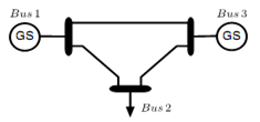 | Figure 1. 3 buses test system |
We consider these assumptions[8]:- The internal field currents are constant, providing the representation of the machine as a constant voltage behind the direct axis transient reactance.- The mechanical power provided by the prime mover is constant and all dynamics of the prime mover are neglected.- All generators are rotating at synchronous speed (steady state) and are round rotors.- All generators in the system are identical, and therefore the inertia is constant (Mi) along with the damping constant (Di) of each generator have the same value.- The mechanical rotor angle is the same as the electrical phase angle of the voltage therefore δ now refers to the electrical angle. To further simplify the notation, the transient reactance is incorporated into the system Ybus, resulting in θi as generator terminal voltage phase and Vi as the terminal voltage magnitude.If we take node 1 as reference, the set of equation of this network is given by[8]: | (2) |
With:  , the node 1 is taken as the reference and :
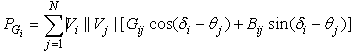 Therefore the model (2) can be rewritten under this form:
 with:
with:  and
and  where u and y will be respectively the control and the output of the system. The choice of transit power as output which is based on this measure is used by the Tunisian Company of Electricity and Gas. Thus for this network, the state vector and the system equations are given by (3) and (4).
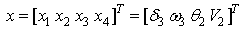 | (3) |
 | (4) |
with x1 and x2 are the dynamic variables, x3 and x4 are the algebraic variables. While using (1) the system is rewritten as:  | (5) |
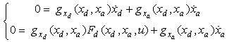
2.2. Semi-explicit DAE index 1
If at an equilibrium point, system (1) is called semi-explicit[10], index-1 property requires that  is solvable for
  and
and  (to simplify
  ):
): | (6) |
Where 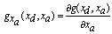 and
and 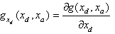 In other words, the differentiation index is 1, if, by the differentiation of the algebraic equations with respect to time, an implicit ODE system results[11]:
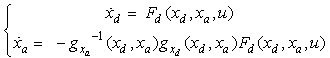 | (7) |
Where 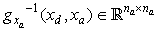 and
and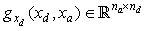 . A study of nature and stability of DAE system is given by[12]. It should be noted that:
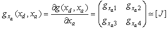 | (8) |
With J is the Jacobian matrix used in the Load Flow calculation excepted for generators terms, which allows us to verify that this  and g is solvable for any
  (the elements of this matrix are the components of the diagonal Jacobian matrix used in load flow).Finally, the complete model in form ODE is as follows:
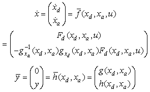 | (9) |
In the expression of  , the purpose of adding the algebraic constraint
  is to check it permanently. It should be noted that the assumptions and the propositions given can be generalized for the other forms of dynamic power system models (models including a characteristic of the static/dynamic loads[9] and generators with exciter model[8]).
3. Fault Detection
The main problem in fault detection[15], based on observer in electrical power system is that few methods are applicable. Effectively, the numerous and strong nonlinearities in presence lead generally to the use of EKF to resolve the fault detection problem. We propose here the EKF, the EKE and the new version of EKF-MH to increase the precision as well as the robustness of the estimation. Hence, a study of the convergence will be presented.
3.1. Extended Kalman Filter
The Kalman filter is a recursive estimator. It means that to consider the running state, only preceding state and current measurements are necessary. The history of the observations and the estimates is; thus; not necessary. In the extended Kalman filter (EKF), the state transition and observation models need not be linear functions of the state but may instead be differentiable functions[13]. The considered nonlinear discrete system is given by (10): | (10) |
Where  and
and  are the system and observation noises which are both assumed to be zero mean multivariate Gaussian noises with covariance
  and
and  respectively.In this paper, we have used the classical form of EKF (we have used Euler discretization with a step size Te,
  to discretize the continuous model (09)) given by:
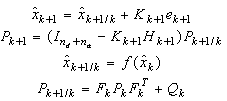 | (11) |
where: 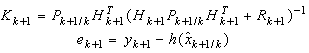 | (12) |
With: 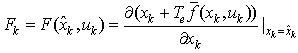 and
and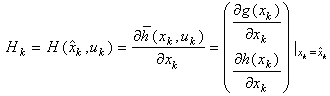 .There are some attempts to apply Kalman Filter on linearized D.A.E system[14], but our proposition is to apply the E.K.E in the classic general form with some numerical approximations that we propose for the Jacobian matrix calculation.Initially, it should be noted that due to the difficulty of finding
  (following the transformation of the algebraic variables in ODE model), we will make the following numerical approximation:
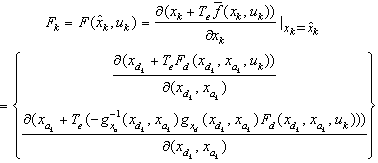 | (13) |
The numerical approximation is used on the second term of  (since it is very difficult to determine) as follows:
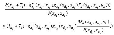 | (14) |
For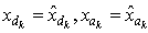 . The terms
  and
and  are calculated numerically. The residual signal is generated by:
3.2. Extended Kalman Estimator
In this section, we present the forms of the most simplified estimator EKE: | (15) |
A simple scalar residual may then be generated by:
3.3. Extended Kalman Filter with Moving Horizon
We propose here the use of an EKF which takes into account a moving horizon of measurements, based on the filter with delay[16], to improve the precision as well as the robustness of estimation. We present in this section the synthesis of the estimator. The proposed observer is given by: | (16) |
With M is a size of moving horizon. In what follows we calculate the various parameters of the filter. We have:  We consider the following approximations:
 We develop
  to obtain:
 | (17) |
Where  .In the expression (17), a total estimation error covariance matrix
  intervenes. This matrix is calculated as follows:
 | (18) |
With in each iteration we must calculate the first component of  with the relation (17). The other elements are calculated by the following expression:
 | (19) |
 | (20) |
We calculate then Kk so as to minimize the trace of error covariance matrix ( ):
): | (21) |
thus, we obtain Kk which satisfies (21):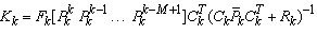 | (22) |
The fact of using a moving horizon to the measures introduces a matrix . The calculation of
 takes into account preceding measures which differ from classical EKF. The initialization of the EKF-MH is given by the EKF in its classical formulation:
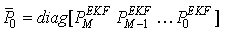 | (23) |
Where  is an estimation error covariance matrix of EKF. In the same way, in the EKF-MH the scalar residual is generated, with the possibility of choosing:
3.4. Convergence Analysis
In this section, we present a convergence analysis of EKE based on the method of[17][18] and[19] by including an unknown diagonal matrix to model linearization errors and a Lyapunov function. This leads to the resolution of a LMI which depends on the choice of Rk and Qk.Briefly, we present some basic steps for EKE and we generalize the results for the EKF and the EKF-MH.Initially, the error vector is defined:  and the candidate Lyapunov function:
  , where :
 We have then:
 | (24) |
A decreasing sequence  means that there exists a positive scalar
  so that:
  .Therefore, the above gives us this LMI:
 | (25) |
With the same reasoning used in[24], we determine domains in which (25) is satisfactory. Under the following assumption: | (26) |
 is a decreasing sequence. With
  and
and  denoting the maximum and minimum singular values respectively, and as
  is a diagonal matrix then:
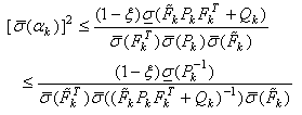 | (27) |
We have then: | (28) |
When (28) is satisfied,  is a strictly decreasing sequence.However, in order to ensure
  and since
  is a strictly decreasing sequence and
  is a bounded matrix, it follows that:
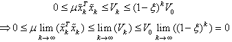 with
with .Consequently, in the same reasoning of[176] and[19], and to guarantee that the EKF, EKE and EKF-MH ensure local asymptotic convergence, we must verify the following conditions:• System (10) is A-locally uniformly rank observable, there exists
  where the observability matrix:
 | (29) |
where:  In practice, we use a numerical rank test on
 .•
.•  ,
,  are uniformly bounded matrices and
  exist.• The matrices Qk and Rk are chosen as follows:i For EKF:
 | (30) |
where  and
and  have to be chosen large and positive and
  and
and  a positive scalar fixed by the user.ii For EKE:
 | (31) |
where  and
and  have to be chosen large and positive and
  and
and  a positive scalar fixed by the user.iii For EKF-MH:
 | (32) |
where: 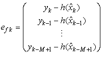 and:
and:  and
and  have to be chosen small and positive and
  and
and  a positive scalar.
4. Simulation Results
Studies are carried out on the IEEE 3 and 13 buses test system to evaluate the performance of the proposed dynamic model and the new observer EKF-MH. The transit power is considered as measurements (we have used the toolbox SimPowerSystems of MATLAB to generate the actual measurements[20]). For the discretization of the model (09), we have used Euler discretization with a step size .
.
4.1. Results of simulation of 3 buses test system
The measurement values are generated by adding low variance noise (±5% of real value) to the generated measurements (transit power P3, 2).We start initially by Fig. 2 which shows the evolution of the rank of the observability matrix (numerical calculation with A=4).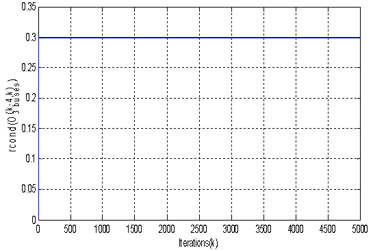 | Figure 2. Evolution of  |
After the verification of the observability,  is well conditioned (
 >0), we present the evolution of
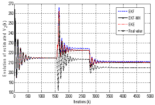
  in Fig. 3 (with a variation of a mechanical power from iteration 2750) after the injection of a defect on the generator node 3,
  (electrical power supplied by the generator) between the iterations 1550 and 1600 with EKF, EKE and EKF-MH (with M=4) where:
 | (33.a) |
 | Figure 3. Evolution of  with standard choice with standard choice |
Figure 3 shows that, with the classical choice of the matrix Rk and Qk , (Standard choice given by (33.a)) the three estimators do not converge to the desired values and then the generated residue is false. We consider, now, the proposed values (Modified choice given by (30), (31) and (32)): | (33.b) |
and we show the variation of  again in Fig. 4:
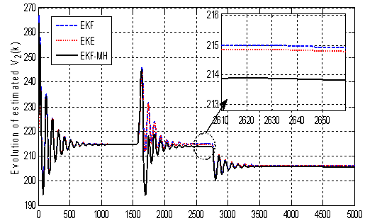 | Figure 4. Evolution of  with the proposed choice with the proposed choice |
The results in Fig. 4 show that the appropriate choice of matrices Qk and Rk given by (33.b) insures the convergence of the estimated states to the real value. We have used a zoom to show the precision offered by the EKF-MH with a small error of 0.02 but with EKF and EKE, it is more than 1.We are interest, now, in the generation and the evolution of the residue signal in the permanent mode.We apply a break line between node 1 and 2 between iterations 1550 and 1700. We show the variation of the residue generated by the three estimators in Fig. 5: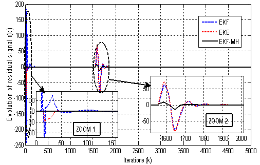 | Figure 5. Evolution of residual signal with EKE, EKE and EKF-MH |
Fig. 5 shows well that the residual signal generated by the EKF-MH gives a variation better than the one given by EKE and EKF at the time of the first iterations (Zoom 1) which can be a false alarm or an indication of a defect. The residual signal generated by EKF-MH indicates only the presence of a defect that varies only in the injection interval default (Zoom 2). This is not the case for the residues generated by the EKE and the EKF. Consequently, the results clearly show the quality of the residue generated by the proposed EKF-MH.
4.2. Results of Simulation of 13 Buses Test System
The network includes: - 5 generators buses: 2, 5, 7, 11 and 12 (with node 12 taken as the reference bus) and 8 static load nodes: 1, 3, 4, 6, 8, 9, 10 and 13.- The outputs are the transit powers between nodes 7 and 6 (P7,6) and nodes 12 and 1 ( ) with a state vector composed by 24 variables (
 with i=2, 5, 7, 11 and j=1, 3, 4, 6, 8, 9, 10, 13).Firstly, we present the evolution of the reciprocal condition estimator
  in Fig. 6 to verify the observability.
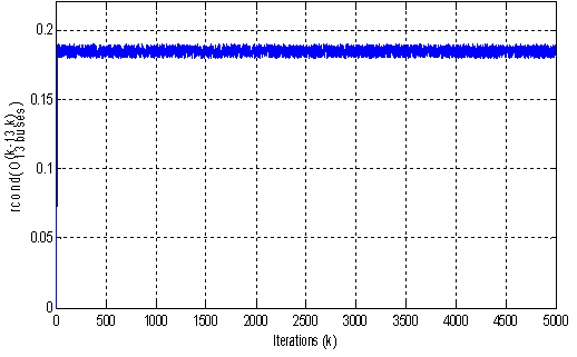 | Figure 6. Evolution of  |
After the verification of the observability,  is well conditioned (
 ), the measurements are generated by applying low variance noise to the measurements (
 of real value). · D1: decrease in the electrical power generator in node 5 (PG5=0) between iterations 1450 and 1700.· D2: break-line between nodes 1 and 13 between iterations 2500 and 2550.· D3: solid three-phase fault to ground applied in node 8 between iterations 2750 and 2850.· D4: short-circuit (single phase-to-ground fault) in node 10 between iterations 4000 and 4020.We show in Fig. 7 the variation of the residual signal generated by the three observers (for EKF-MH M=10):Fig. 7 shows clearly that the variation of the residue generated by the EKF-MH remains limited in the injection interval of defect and it is the only one which can indicate the presence of two defects D2 and D3 (Zoom 2). However with the EKE and EKF, the residual signal indicates the presence of a single defect. In the same way of 3 buses test system and in the first iterations, the EKF and the EKE generate false indication of defects (Zoom 1).We are interested in the convergence of the three observers (EKF-MH, EKE and EKF). The measurement values are generated by adding high variance noise to the measurements ±15% of real value). We consider:· The classical values of Qk and Rk given by (Standard versions: S-EKF-MH, S-EKF and S-EKE):
 | (34.a) |
· Modified proposed values given by (34.b): Modified versions based on the proposed conditions (30), (31) and (32); M-EKF-MH, M-EKF and M-EKE: | (34.b) |
We consider 100 simulations while varying the initial values in a random way (variation of ±20% with respect to the actual initial values) and we present in table 1 the rate of convergence:| Table 1. (%) of Convergence with random initial values |
| | Observers | (%) of convergence | | S-EKF | 42 % | | M-EKF | 82 % | | S-EKE | 48 % | | M-EKE | 86 % | | S-EKF-MH | 64 % | | M-EKF-MH | 98 % |
|
|
Table 1 gives a clear idea about the convergence of the proposed EKF-MH. As we can see (line 6 of Table 1), the modified EKF-MH converges with an accurate precision (in the majority of cases, 98%) more than other observers. However, the modified versions of EKF and EKE can improve the rate of convergence. I one word, many results are omitted.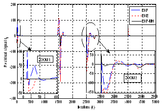 | Figure 7. Evolution of residual signal with EKE, EKE and EKF-MH |
5. Conclusions
In this paper an observer based approach for a fault detection is presented. A new filter design based on fundamental problem of residual generation concepts has been elaborated for nonlinear dynamic power system.An EKF-MH has been described and investigated based on a moving horizon to generate a perfect residual signal to fault detection. We have also used the classical design of EKF and EKE by including some numerical approximation for the calculation of Jacobian matrix which was preceded by a convergence analysis. Numerical results demonstrate the potential of this approach in failure detection and show well the advantage of the proposed choice of Rk and Qk in terms of robustness and convergence. In a very clear way, this approach presents a good quality of fault detection with a combination of successive and simultaneous injection of the majority of real types of defects. Experimental verification is, then, a necessity to testify the practical performance of this approach in the near future.
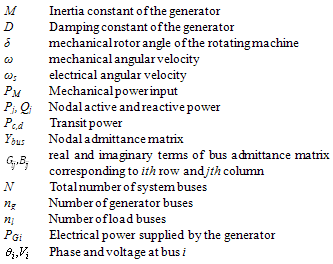
Nomenclature
References
| [1] | Y. Chetouani. “Using the kalman filtering for the fault detection and isolation (FDI) in the nonlinear dynamic processes”. Int .J. of Chem. Reactor Eng. Vol. 6, pp. 1-20, 2008. |
| [2] | X. Zhang, T. Parisini, M. Polycarpou. “Sensor bias fault isolation in a class of nonlinear systems”. IEEE Trans.on Auto. Control. Vol. 50, pp. 370-376, 2005. |
| [3] | J. Stoustrup, H. Niemann. “Fault detection for nonlinear systems-a standard problem approach”. IEEE Conference on Decision and Control. Tampa, Florida, USA, pp. 96-101, 1998. |
| [4] | J.J R. Pasaye, R. G. Lopez. “Fault diagnosis in nonlinear systems: An application to a three-tank system”. Proc. American Control Conference, Seattle, Washington, USA, pp. 2136-2141, 2008. |
| [5] | D.F. Leite, M.B. Hell and P.J.F. Gomide. “Real-time fault diagnosis of nonlinear systems”. Int. Multidisciplinary J. on Nonlinear Analysis. Vol. 71, pp. 2665- 2673, 2009. |
| [6] | A. Shumsky. “Robust analytical redundancy relations for fault diagnosis in nonlinear systems”. Asian Journal of Control. Vol. 4, pp. 159-170, 2002. |
| [7] | J. Chen, R.J. Patton. Robust Model-Based Faults Diagnosis for dynamic systems. Dordrecht: Kulwer, Academic Press, 2nd edition, 1999. |
| [8] | C.J. Dafis. An observability formulation for nonlinear power systems modeled as differential algebraic systems. Ph.D. dissertation, Drexel University, PA, USA, 2005. |
| [9] | D. Karlsson and D.J. Hill. “Modelling and identification of nonlinear dynamic loads in power systems”. IEEE Trans. on Power Syst. Vol. 9, pp. 157–166, 1994. |
| [10] | T. Wichmann. “Simplification of nonlinear DAE systems with index tacking”. European Conf. on Circuit Theory and Design, Espoo, Finland, pp. 173–176, 2001. |
| [11] | B.W. Gordon. “Dynamic sliding manifolds for realization of high index differential-algebraic systems”. Asian J. of Control. Vol. 5, pp. 454–466, 2003. |
| [12] | D.C. Tarraf and H.H. Asada. “On the nature and stability of differential-algebraic systems”. Proc.American Control Conf., Anchorage, Al USA, pp. 3546–3551, 2002. |
| [13] | K. Judd. “Nonlinear state estimation, indistinguishable states, and the extended kalman filter”. Physica D: Nonlinear Phenomena. Vo. 183, pp. 273–281, 2003. |
| [14] | V.M. Becerra, P.D.Roberts, and G.W. Griffiths. “Applying the extended kalman filter to systems described by nonlinear differential-algebraic equations”. Control Eng. Practice. Vol. 9, pp. 267–281, 2001. |
| [15] | K. Gark, L. Weingarth, S. Shah. “Dynamic positioning power plant system reliability and design”. Europe Conf. Proc. Petroleum and Chemical Industry (PCIC Europe), Rome, Italy, pp. 1-10, 2011. |
| [16] | M. Boutayeb. “Observers design for linear time-delay systems”. Syst. and control Lett. Vol. 44, pp. 103–109, 2001. |
| [17] | M. Boutayeb and C. Aubry. “A strong tracking extended kalman observer for nonlinear discrete-time systems”. IEEE Trans. on Autom. Control. Vol. 44, pp. 1550–1556, 1999. |
| [18] | M. Boutayeb. “Identification of nonlinear systems in the presence of unknown but bounded disturbances”. IEEE Trans. on Autom. Control. Vol. 45, pp. 1503–1507, 2000. |
| [19] | Y. Song, J. Grizzle. “The extended kalman filter as a local asymptotic observer for nonlinear discrete time sys tems”. J. Math. Syst. Estimation and Control. Vol. 5, pp. 59-78, 1995. |
| [20] | A. Thabet, M. Boutayeb, M.N. Abdelkrim. “Real time dynamic state estimation for power system”. Int. J. Computer Applications. Vol. 38, pp. 11-18, 2012. |
 Abstract
 Reference
 Full-Text PDF
 Full-text HTML