1. Introduction

The Distributed generations (DGs) are small-scale power generation technologies of low voltage type that provide electrical power at a site closer to consumption centres than central station generation. It has many names like Distributed energy resources (DER), onsite generation, and decentralized energy. DGs are from renewable and artificial models. DGs are the energy resources which contain Renewable Energy Resources such as Wind, Solar and Fuel cell and some artificial models like Micro turbines, Gas turbines, Diesel engines, Sterling engines, Internal combustion reciprocating engines[1]. In the present vast load growing electrical system, usage of DG have more advantages like reduction of transmission and distribution cost, electricity price, saving of the fuel, reduction of sound pollution and green house gases. Other benefits include line loss reduction, peak shaving, and better voltage profile, power quality improvement, reliving of transmission and distribution congestion then improved network capacity, protection selectivity, network robustness, and islanding operations[2-3]. The impact of DG on power losses is not only affected by DG location but also depends on the network topology as well as on DG size and type[1]. The placement, type and size of the DG should be optimal in order to maximize the benefits of it[4]. For optimal placement of the DG in Distribution system, evolutionary methods have been used, as they can allow continuous and discrete variables[5-6]. Many analytical approaches[7-9] are available for optimal DG, but they cannot be directly applied, because of the size, complexity and the specific characteristics of distributed systems[1]. In[7,8,10-12] the optimal placement and size of single DG was considered and in[9,13-15] optimal placement and size for multi DGs were determined. In all these papers the bus available limit is not considered for placement of DG. The main objective of this paper is to optimize the power system modelled multi DGs location and size, while minimizing system real, reactive losses and to improve voltage profile and line loading by considering the bus available limit of the Renewable DGs like wind mills and Photovoltaic. The renewable energy DGs placement is limited to a number of busses with the consideration of environmental constrains.

2. Impact Indices and Objective Function

2.1. Impact Indices

2.1.1. Real and Reactive Loss Indices (ILP and ILQ)

The active and reactive losses are greatly depending on the proper location and size of the DGs. The indices are defined as

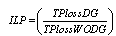(1)

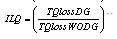(2)

Where, TPlossDG and TQlossDG are the real and reactive power losses of the distribution system with DG. TPlossWODG and TQlossWODG are the real and reactive power losses of the system without DG.

2.1.2. Voltage Profile Index (IVD)[15]

The voltage profile of the system is depending on the proper location and size of the DGs. The IVD is defined as

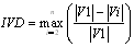(3)

Where n is the number of busses in system. V1 is the substation bus voltage (reference voltage). V_i is the i^th bus voltage.

2.1.3. MVA Capacity Index (IC)[15]

The IC index gives the important information about the line of MVA flow through the network regarding the maximum capacity of conductors. The IC can be defined as

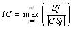(4)

Where nl is the number of lines (branches) in system. Sj is the j^th line flow and CSj is the maximum capacity of the j^th line flow. This index penalises the size and location pair which gives higher flow deviation of the line from the MVA capacity of the line. Hence make the uniform line flows in the system without congestion.

2.2. Objective Function

The main objective of this paper is to study the effect of placing and sizing the DG in all system indices given previously. Also observe the study with renewable bus available limits. Multi objective optimization is formed by combining the all indices with appropriate weights. The multi objective function is defined as

(5)

In this paper the weight are considered as W₁=0.4, W₂=0.2, W₃=0.25 and W₄=0.15 and fallowing the constraint

where

The weights are indicated to give the corresponding importance to each impact indices for the penetration of DGs and depend on the required analysis. In this analysis, active power losses have higher weight (0.4), since the main importance is given to active power with integration of DG. The least weight is given to the IVD, since the IVD is normally small and within permissible limits. The OF(5) is to minimize with equality and inequality constraints.

Equality constraint is

(6)

In equality constraint is

(7)

3. Modelling of DGs in Load Flow Studies

In system with DGs, the generation of Photo voltaic systems, Fuel cells, Microturbines and some Wind turbine units are injected into the power grid via power electronic interfaces. In such cases, the model of a DG unit in load flows depends on the control method which is used in the converter control circuit. The DGs which have control over the voltage by regulating excitation voltage (Synchronous generator DGs) or the control circuit of the converter used to control ‘P’ and ‘V’ independently, then the DG unit may be model as PV type. Other DGs like Induction generator based units or converter used to control P and Q independently, then the DG shall be modelled as PQ type. Using these models for DGs, Current injection based load flow method is employed for Distribution system studies.

3.1. DG Modelled as PQ Node

A DG unit can be modelled as three different ways in PQ node mode as illustrated below:

3.1.1. DG as a ‘Negative PQ Load’ Model of PQ Mode

In this case the DG is simply modelled as a constant active (P) and reactive (Q) power generating source. The specified values of this DG model are real (P_DG) and reactive (Q_DG) power output of the DG. It may me noted that Fuel cell type DGs can be modelled as negative PQ load model. The load at bus-i with DG unit is to be modified

(8)

(9)

3.1.2. DG as a ‘Constant Power Factor’ Model of PQ Mode

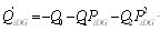
The DG is commonly modelled as constant power factor model[16]. Controllable DGs such as synchronous generator based DGs and power electronic based units are preferably modelled as constant power factor model. For example, the output power can be adjusted by controlling the exciting current and trigger angles for synchronous generator based DGs and power electronic based DGs, respectively[16]. For this model, the specified values are the real power and power factor of the DG. The reactive power of the DG can be calculated by (10) and then the equivalent current injection can be obtained by (11)

(10)

(11)

3.1.3. DG as ‘Variable Reactive Power’ Model of PQ Mode

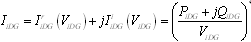
DGs employing Induction Generators as the power conversion devices will act mostly like variable Reactive Power generators. By using the Induction Generator based Wind Turbine as an example, the real power output can be calculated by Wind Turbine power curve. Then, its reactive power output can be formulated as a function comprising the real power output, bus voltage, generator impedance and so on. However, the reactive power calculation using this approach is cumbersome and difficult to calculate efficiently. From a steady-state view point, reactive power consumed by a Wind Turbine can be represented as a function of its Real Power[17], that is

(12)

Where Q’iDG is the Reactive Power function consumed by the Wind Turbine. The Q₀, Q₁ and Q₂ are usually obtained experimentally. The reactive power consumed by the load cannot be fully provided by the distribution system, and therefore capacitor banks are installed for power factor correction where induction generator based DGs are employed.

3.2. DG Modelled as PV Type

The DG as a PV node is commonly Constant voltage model. The specified values of this DG model are the real power output and bus voltage magnitude. For maintain constant voltage the, change in voltage ΔVi should maintain zero by injecting required reactive power.

3.3. Modelling of WIND and SOLAR DGs

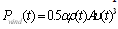
The Photovoltaic systems convert Solar Energy into Electrical energy. Their output is DC power and is converted into AC power via an inverter to be compatible with AC grid. The power output of a solar photovoltaic (PV) panel depends on the area (A) of the PV panel, solar irradiance μ(t) and efficiency of the PV panel β[18]

(13)

The Wind turbine power output[18] is proportional to the kinetic energy, air density, etc. Other parameters of Wind turbine include cut- in wind speed, cut-out wind speed and rated wind speed, and typical values of them are 3.5 m/s, 25 m/s, and 14 m/s respectively. Precise values can be obtained from manufacturer’s data sheet for the respective limits.

(14)

Where α is the Albert Betz constant, ρ(t) is air density, A is area swept by turbine rotor, and ν(t) is wind speed[18]. The energy sources of DGs can be categorized into stable and unstable energy sources, Fuel cell and Micro-gas turbine are some of the stable energy sources, Wind and Solar are most commonly used unstable energy sources. Different energy sources show special output characteristics when combining with different energy converters[16]. For example, the Induction Generator will act like a constant real power and variable reactive power generator, when it is used to convert wind energy to power grids. So it is modelled as a variable reactive power model in load flow analysis. However, if the static electronic converter is used to convert Solar to power grids, it will mostly act like a generator with a constant power factor in normal operating condition. Therefore it is modelled as constant power factor model. The maximum power rating of Solar photovoltaic station is fixed by taking average of total day solar powers calculated by using equation (13). Similarly maximum power rating of wind station is fixed by taking averages of all day powers calculated by using equation (14). In this study, the maximum capacity of DG is taken as 0.63 p.u and for renewable DGs like Solar and Wind is calculated from the average power estimated by irradiance and wind speed respectively. The table.1 shows the data of solar irradiation[19] over 24 hours and wind speed data[20]. Calculate the power generated for every irradiance level and wind speed by using the equations (13) and (14) respectively. In this study the average power generated by the Solar is 1.191p.u and Wind turbine is 0.471p.u.

Table 1. Solar and Wind Data for 24 hours Time (hours) Solar irradiance Data (W/m2) Wind speed Data(m/sec) 1 0 3.0335 2 0 3.5412 3 0 4.9334 4 0 5.7063 5 0 6.5247 6 32.1779 6.3937 7 203.3411 5.256 8 406.6817 3.6345 9 575.9177 4.1387 10 733.1582 4.5555 11 872.7758 4.3235 12 737.8383 4.0157 13 815.881 2.7205 14 818.2873 2.6466 15 732.5975 3.9623 16 565.549 3.4079 17 455.1528 5.3587 18 139.9814 6.0713 19 37.669 5.2234 20 0 4.8908 21 0 2.1175 22 0 1.7315 23 0 4.7083 24 0 4.9598

4. GA Implementation for Optimal Placement and Size of DG

In this paper Genetic algorithm based optimization technique is used to find the optimal placement and size of the DG by minimizing the losses and voltage improvement. The simple GA contains chromosome size of 20 bits for every DG. In that 20 bits 8 are for placement of the DG and remaining 12 are for Size of the DG. The formation of chromosome is shown in fig.1. Population size of 120 and Elitism operator of 0.1, Crossover probability of 0.7 and mutation probability 0.005 are used in this work. Maximum numbers of iterations are 500.

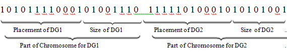Figure 1. Chromosome formation of DGs

5. Results and Validation

For testing the proposed study, the test data of 38 Bus Distribution Systems are considered. System data of 38 bus Distribution systems are available in paper[21].

5.1. Case-I: 38 Bus Distribution Systems with No Bus Available Constraints

This case study include various combination of different distribution generation units like: without DG, Solar, Wind, Fuel cell, Micro turbine, combination of Solar and Wind; Solar, Wind and Fuel cell; Solar, Wind, Fuel cell and Micro turbine. Here, the Solar is modelled as a constant power factor model, Wind is modelled as a Variable reactive power model, Fuel cell is modelled as a negative real power load model and Micro turbine is modelled as a constant voltage model in load flow studies. This study includes various combinations of different distribution generations, which are clearly tabulated and presented for 38 bus distribution bus system. Table 2 shows the optimal placement of DGs and its corresponding sizes and active and reactive power losses for different combination of DGs to 38 bus distribution system. It is found that without DG the losses are 20.2 kW and 13.4847 Kvar. There is significant reduction in losses in case of Solar Photovoltaic DG integration when compared to Wind turbine DG. This is because of the maximum available rating of Solar is 2.52 times more than Wind turbine power rating.

The losses are reduced 89.1% with integration of all available four DG case. In this study the losses margin is very less in 3 DGs integration compared to 4 DGs integration. Which instigates that number of DGs should be limited to four taking into consideration the initial and maintenance cost.

Table 3 gives the ILP, ILQ, IC, IVD and OF for all cases of 38 bus distributed systems. In all combination of DGs cases the IVD is nearer to zero. It means that the voltage profile is improved and voltage deviation observed is very small. It is observed that ILP, ILQ, IC and IVD all are reducing with increasing the number of DG integration case, where as the variation rate is small in case of three DGs and four DGs combination cases. Objective function is reduced 46.4% with combined integration of all four DGs compared to single DG (Fuel cell) case.

From figure 2, it is observed that the voltages are improved with optimal placement and appropriate size of the DGs. It is observed that, with the integration of the four available DGs the voltage profile is improved significantly. It is also observed that by increasing the number of DGs the voltage profile is improving. At low voltage (13,14,15,16,17, 18,30,31,32,33,36 and 38) busses the significance of DG integration is clearly observed . Whereas the improving rate of voltage is decreased by increasing the DG numbers. So it is clearly observed that for this case study the number of DGs is limited to four.

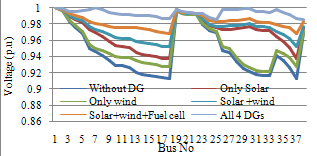Figure 2. Voltage profile with combination of DGs in 38 bus system without renewable DG bus available limit

Table 2. Optimal Place and Size of the DG in 38 Bus system without renewable DG bus available limit S.No various combination of Distribution generations Optimal DG BUS Number DG Value(*100kW)/ reactive power(*100kVAR) required for Wind mills Active power loss (*100kW) Reactive power loss (*100kVAR) 1 Without DG NO DG NO DG 0.2022 0.13484 2 Only Solar 30 1.191/0.61016 0.0813 0.05638 3 Only Wind 13 0.471/0.252478 0.1765 0.11746 4 Only with Fuel Cell 14 0.63 0.1428 0.09455 5 Only Micro turbine 30 0.63/2.515639 0.1421 0.10037 6 Solar +wind 30(solar) 1.191/ 0.610167 0.0698 0.04824 14(wind) 0.471/ 0.252478 7 Solar+ Wind+Fuel cell 30(solar) 1.191/ 0.610167 0.0448 0.03107 25(wind) 0.471/ 0.252478 13(Fuel cell) 0.63 8 Solar+ Wind+Fuel cell+ Microturbine 30(solar ) 0.991449 /0.572172 0.0222 0.01668 24(wind) 0.47002/ 0.252478 15(Fuel cell) 0.630000 7(M-turbine) 0.63/ 1.051823

Table 3. Performance Indices for 38 bus system without renewable DG bus available limit Only Solar Only Wind Only Fuel cell Only Micro turbine Solar + wind Solar+ wind+ Fuel cell All 4 DGs ILP 0.402 0.8729 0.7065 0.703 0.3455 0.2216 0.1098 ILQ 0.418 0.871 0.7012 0.744 0.3577 0.2304 0.1237 IC 0.9995 0.9951 0.9951 1.132 0.995 0.9854 0.9854 IVD 0.06237 0.0784 0.0733 0.053 0.0478 0.0308 0.01476 OF 0.5037 0.7839 0.6826 0.721 0.4656 0.3857 0.3172

5.2. Case-II: 38 Bus Distribution System with Bus Available Limits

The busses which are connected to solar power generation and wind power generation mainly depend on the environmental conditions. In this study, for investigational purpose the available renewable DG bus numbers are purely assumed. The Solar DG busses are limited to 17 to 22 busses and Wind DG busses are limited to 27 to 33 busses. The other, not nature dependent DGs like micro turbine and Fuel cell are can be placed in any bus in the system. The process of limiting busses is done by limiting the search area of chromosome in GA for the DG integration bus to available bus limits. Fig 3 shows the 38 bus distribution system and assumed bus limits for wind and solar availability.

Table 4 shows the optimal placement and size of the different combination of DGs and losses of the system. In this case the solar and wind DGs are limited to available busses. The losses are increased compared to the case-1(no bus limits case). The DG bus available constraint make the optimization algorithm to lower search space, hence the losses are not reduced compared to previous full search area case-1. In this case losses are reduced with integration of all available four DGs.

Table 5 shows the different indices and objective function of the 38 bus distribution system with bus availability constraints. All the indices and OF values in all combination of DG units are greater than the previous case-1. It is clearly shown that because of the renewable DG available busses are limited, all indices are raised and the system not used the full affect of the DGs. The OF is reduced 15.48% with combined integration of all Four DGs compared to single DG(Fuel cell) integration and compared to previous case-1 it is increased from 0.317 to 0.704. The voltage profile with bus available limits consideration is shown in fig 4.

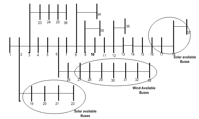Figure 3. 38 bus distribution system with assumed bus limits for wind and solar availability

Table 4. Optimal Place and Size of the DG in 38 Bus system with renewable DG bus available limit S.No various combination of different Distribution generations Optimal DG BUS Number DG Value(*100kW)/ reactive power(*100kVAR) required for Wind mills Active power loss (*100kW) Reactive power loss (*100kVAR) 1 Without DG NO DG NO DG 0.202212 0.134847 2 Only Solar 17 0.364923 0.149231 0.098707 3 Only Wind 27 0.66/0.252478 0.176100 0.118665 4 Solar + wind 17(solar) 0.3649/ 0.186956 0.129593 0.086721 27(wind) 0.66/ 0.330516 5 Solar+ Wind+Fuel cell 17(solar) 0.3649/ 0.18685 0.096453 0.064241 27(wind) 0.5515/ 0.2927 31(F-cell) 0.63 6 Solar+ Wind+Fuel cell+ Micro turbine 17(solar ) 0.36268 / 0.18580 0.029911 0.021053 28(wind) 0.47002/ 0.252478 11(F-cell) 0.570923 29(M-turbine) 0.63/ 1.428885

Table 5. Performance Indices for 38 bus system with renewable DG bus available limit Only Solar Only Wind Only Fuel cell Only Micro turbine Solar + wind Solar+ wind+ Fuelcell All 4 DGs ILP 0.888 0.979 0.956 0.999 0.872 0.832 0.831 ILQ 0.890 0.979 0.957 0.998 0.875 0.835 0.833 IC 0.961 0.987 0.981 0.823 0.955 0.943 0.770 IVD 0.086 0.092 0.092 0.094 0.086 0.082 0.082 OF 0.787 0.8484 0.833 0.819 0.776 0.748 0.704

Fig 4 shows the improvement in the voltage profile under different combination of DGs. As shown in the figure, the voltages at all busses improved significantly with integration of all 4 DGs. In all two cases, with the insertion of the 4 DGs there is no more change in the voltage profile. With the Renewable DG integration there is significant reduction of the voltage at sensitive busses (15, 16, 17, 18, 37 and 38) from case-1 to case-2. The effect of the renewable DG available limit in voltage profile of the system is reduced with increasing the number of Renewable and non renewable DGs.

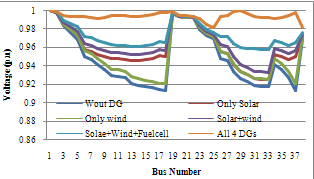Figure 4. Voltage profile with combination of DGs in 38 bus system with renewable DG bus available limit

6. Conclusions

The placement and size of the DGs with Different DG models considering their bus available limits in a 38 bus distribution system was presented. The objective function, which contains the different objectives combined with weights, is optimized with and without considering the DG available bus limit constraints. The different impact indices, losses and voltages profile at all busses are studied at all cases.