E. C. Merem 1, Y. A. Twumasi 2, S. Fageir 3, D. Olagbegi 1, J. Wesley 1, R. Coney 1, Y. Babalola 1, T. Thomas 1, A. Hines 4, G. Hirse 4, G. S. Ochai 5, E. Nwagboso 6, M. Crisler 1, S. Leggett 7, J. Offiah 1, S. Emeakpor 8
1Department of Urban and Regional Planning, Jackson State University, 101 Capitol Center, Jackson, MS, USA
2Department of Urban Forestry and Natural Resources, Southern University, Baton Rouge, LA, USA
3Department of Social Sciences, Alcorn State University, 1000 ASU Drive, Lorman, MS, USA
4Department of Public Policy and Administration, Jackson State University, 101 Capitol Center, Jackson, MS, USA
5African Development Bank, AfDB, 101 BP 1387 Avenue Joseph Anoma, Abidjan, AB 1, Ivory Coast
6Department of Political Science, Jackson State University, 1400 John R. Lynch Street, Jackson, MS, USA
7Department of Behavioral and Environmental Health, Jackson State University, 350 Woodrow Wilson, Jackson, MS, USA
8Department of Environmental Science, Jackson State University, 1400 John R. Lynch Street, Jackson, MS, USA
Correspondence to: E. C. Merem , Department of Urban and Regional Planning, Jackson State University, 101 Capitol Center, Jackson, MS, USA.
| Email: |  |
Copyright © 2024 The Author(s). Published by Scientific & Academic Publishing.
This work is licensed under the Creative Commons Attribution International License (CC BY).
http://creativecommons.org/licenses/by/4.0/

Abstract
The state of Maryland for all intents and purposes stands out as a pacesetter in different aspects of environmental planning more than other states. Known for having the first established planning commission in the United States decades ago before its neighbors and a longstanding tradition in orderly planning. One would think such illustrious trajectory, that Maryland enjoys, guarantees immunity from common exposures to climate change dangers based on experience. However, that is not really the case in the Mid Atlantic zone. The same state that boasts of some of the most successful farming operations and a flourishing economy heavily reliant on a stable ecosystem, now finds itself at the receiving end of climatic uncertainty along the coast. Accordingly, the lower side of Maryland has seen full share of climate change induced threats like ice storms, floodings and elevated temperature. All these results in widespread damage to society, economy, and the surrounding ecosystem, amidst the vulnerability of many sectors. The situation in the coastal environment is compounded by sea level rise, potential displacements, degradation, destruction of assets and anticipated inundation of low-lying settlements in the coming years. Notwithstanding the gravity of these issues, very little has been done to capture the risks sufficiently in the literature. Consequently, this enquiry will fill that void notably by analyzing the changing climate risks in Southern Maryland using mix-scale methods of GIS and descriptive statistics. Emphasis is on the trends, issues, factors, impacts and efforts towards containment of the hazards. Accordingly, the results of the trends show widespread risks exposure through periodic damages to the ecosystem, along with fiscal losses in some sectors of the economy. With all these attributed to ecological, socio-economic, policy and climatic uncertainty. The paper proffered solutions ranging from education, the strengthening of policies, the design of regional climate information system and the recourse to coastal zone planning.
Keywords:
Climate change, Ecosystem, Coastal environments, Sea level rise, GIS, Region, Policy, Degradation
Cite this paper: E. C. Merem , Y. A. Twumasi , S. Fageir , D. Olagbegi , J. Wesley , R. Coney , Y. Babalola , T. Thomas , A. Hines , G. Hirse , G. S. Ochai , E. Nwagboso , M. Crisler , S. Leggett , J. Offiah , S. Emeakpor , The Analysis of Extreme Climate Threats in Maryland’s Lower Region Along the US Mid Atlantic, World Environment, Vol. 14 No. 1, 2024, pp. 1-19. doi: 10.5923/j.env.20241401.01.
1. Introduction
The state of Maryland [1], for all intents and purposes stands out as a pacesetter in different aspects of environmental planning more than the other states. Known for having the first established planning commission in the United States decades ago before its neighbors. The state has a longstanding tradition in orderly planning. For that, one would think that such illustrious history which Maryland enjoys, guarantees the state immunity from common exposures to climate change dangers based on experience. However, that is not really the case in the Mid Atlantic zone [2]. Accordingly, in the past years, Maryland’s climate has been shifting to hotter and wetter conditions amidst recurrent pace of severe weather incidents. Temperatures have also already risen by about 2.5°F, as the number of very hot days keeps increasing [3]. According to the thermal index, the summer periods in the zone continues to be hot due to rising temperature often deemed as a major cause of fatalities, and an element fuelling ground-level ozone, a critical health risk. For that, by 2050, the usual duration of heat wave periods in Maryland, is expected to jump considerably by over several days annually [4,5]. Said that, this trend has quickened the probability of climate induced disasters to the extent that, the Chesapeake Bay is now listed among the most susceptible areas to climate change impacts via elevated temperature and shifts in ecological conditions [6,7]. Against that background, the mean yearly rainfall has also risen, and rainstorms are predicted to surge with reoccurrence and ferocity. Also, the seasons are turning out to be less distinct as warmer winters, and rising sea levels persist at 1 inch every 5 years. For that, higher water flows are rapidly washing away beach fronts, sinking low lying areas while intensifying coastal flooding, and driving up the saltiness of creeks and aquifers with risks to human and natural ecosystem in the study area. Overtime, the changing climate will likely accelerate shoreline and inland flooding; with damages to marine and inland ecosystems, while interrupting fishing and agriculture [8-11]. The same state that boasts of some of the most successful farming operations and a flourishing economy heavily reliant on a stable ecosystem, now finds itself at the receiving end of climatic uncertainty along the coast [12-14]. Accordingly, the lower side of Maryland has seen full share of climate change induced threats like ice storms, floodings and elevated temperature. Since all these are resulting in widespread damage to society, economy, and the surrounding ecosystem, amidst the vulnerability of many sectors. The state has now become an area where about 110,000 people, face the vulnerability to extreme heat, as other places including the Southern region are burdened by 10 days of risky heat levels based on a projected period of 40-50 days in extreme heat annually by 2050 [15]. With that has come climate change induced nuisance floodings in Maryland [16-18]. To that effect, by 2005-2014, the Annapolis area saw over 394 total floods with 75% of that, human induced [19-21]. The situation in the coastal environments is compounded further by the growing intensity of sea level rise, potential displacements of people, degradation, destruction of assets and anticipated inundation of low-lying settlements in the coming years [22,23]. This is occurring in the face of forest disturbance triggered by urban development in the big counties in ways likely to threaten the role of woodlands as emission sinks [24]. As such, today in Maryland, 81,000 citizens share coastal flooding exposures and by 2050, an additional 38,000 citizens are projected to be at risk, as submergence looms over cities. In all these, deadly Atlantic hurricanes continue to hit coastal areas in the South with more category 5-6 Atlantic hurricanes said to have landed between 1970-2010. Of the 84.3 million gallons of sewage spilled in Maryland after Hurricane Sandy in 2013, 82% of the overflows came from runoffs. The rising pace of sea level in the process, has resulted in severe coastal erosion, sedimentation, and flooding with mitigation price tag of nearly $3b. This is evident with surges in tidal flooding in Maryland at the rate of 178% since 2000. While this pushed up liability levels of assets, it resulted in the exposure of over 3,000 properties to high risks category despite all current efforts in place. In that way, the ferocity of climate change hazards stands as a major concern [3,4,25]. In that setting, the flooding of roadways, suspension bridge, tunnels, and other highways, disrupts daily activity in every part of affected areas. This not only stalls the movements of crisis and first responder cars and individuals heading to workplace places and schools. But flooding events of such magnitude constitutes an impediment to the operations of local markets essential to community life. Being a state reputed for the heavy concentration of human settlements and natural areas stretching from big towns to flourishing beach front municipalities. The presence of these assets on terrains at high propensity to torrential flooding beyond the specified flood zones, puts them in jeopardy. This is especially the case in inland areas not accustomed to recurrent inundation [9]. The disparate costs in home insurance for coastal residents and tens of thousands of citizens living in areas below 6 feet along shorelines, compounds the matter. Furthermore, the presence of CO2 emitting facilities in the counties and carbon footprints therein constitutes major worry [26-34]. Despite the gravity of these issues, little has been done to capture the risks sufficiently in the literature. This enquiry will fill that void by analyzing the climate change risks in Southern Maryland using mix-scale methods of GIS and descriptive statistics [35-40]. Emphasis is on the trends, issues, factors, impacts and efforts towards mitigation [41-46]. The study has five objectives. The first aim consists of the use of geo-spatial tech to analyze the status of climate issues and changes, while the 2nd objective is to offer a support tool for policy makers. The third goal stresses the design of a fresh method for systematizing climate change index. The fourth aim is to craft a framework for regional ecological impact analysis. The fifth aim is to assess climate risk trends. Accordingly, the study covers 5 sections consisting of introduction, methods, results, discussions, and conclusion.
2. Methods and Materials
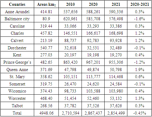
The study area Southern Maryland [Fig. 1] which stretches through 14 counties is the state's most ecologically viable landscape. With a population of more than 2.8 million in 2021 (Table 1), the larger region with 72% of the citizens of the state, occupies a land area of 4,986 miles to 3,100 miles in shorelines often under heavy risks from climate variability [4]. In the same vein, Maryland occupies the 35th position nationwide on CO2 discharges with 48.1MMT emissions in 2020. Located in a state ranked 4th nationwide as the most at-risk area facing the impacts of climate change induced sea-level rise. In that light, accelerated sea levels and surge in storm power have the capacity to unleash arduous repercussions on South Maryland’s coastline. The same goes for the Chesapeake Bay ecozone now at a scale likely to endanger the ecological, leisure, and fiscal fortunes revered by citizens and tourists drawn by the charm of the zone [47-50]. Table 1. Population and area of Study Area
 |
| |
|
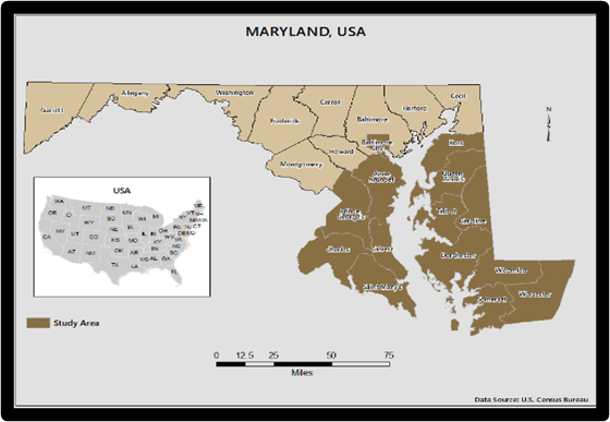 | Figure 1. The Study Area Maryland Southern Region |
Aside from all its attributes, the Southern Maryland region boasts of among many other things one can think of. This includes much of the country’s oldest known first communities, and the most preferred due to the closeness to water and secured ports, rich soils, and plentiful wildlife. Until the 1960's, Southern Maryland stood out as a terrain overshadowed by flourishing farming operations. Nowadays, the zone remains a hub of vast swaths of major farmlands but has now diversified into new areas through enlarged network of opportunities amidst thriving activities in a whole range of sectors from wineries, breweries together with exceptional business rooted in sustainability. Notwithstanding a surge in the number of households and a population of millions citizen beginning in the 1940's, the Southern Maryland region still stands out among the major ecologically treasured sites statewide today [51-55]. Dubbed as a sanctuary to multiplicity of amphibian, freshwater fish species, filled with migratory and shoreline bird types. The study area is also highly ranked ahead of others regarding the plethora of environmental functions it performs in the natural setting. Accordingly, South Maryland’s ecozone remains a vital sanctuary to rich amphibian and freshwater fish species and migratory and coastal birds. Being the state’s treasured ecosystem, the Chesapeake Bay ranks high for its diverse flora and fauna and biodiversity refuge. While other components of the region's ecosystem consist of freshwater and terrestrial systems from tidal marshes, forests, and coastal systems like coral reefs off the Atlantic coast [4]. In terms of species and vastness of marshes along the Bay’s region, look no further than the landscape in the Lower Dorchester County, Maryland, especially at the Blackwater National Wildlife Refuge that is full of habitats for biodiversity. Granted the presence, the loss of tidal marshes threatens both life, shelter and food source for birds and fish. Based on climate change risks, both the Bay’s ecozone and built-up areas are now endangered [Fig. 1.1]. Within the low side of the landscape, Dorchester’s tidal marshes are the epicenter of the shifting climate effect on the Chesapeake Bay. For that, there are concerns over how new sediment flows emanating from floods as the projected damage from the tidal marsh, threatens the region’s-built environment and salt marsh flora and fauna [56-58]. Realizing the significance of ecological services of tidal marshlands, and the challenges faced from changing climate locally. Organizations like the Southern Maryland Conservation Alliance have been in the forefront of efforts to conserve and restore areas at risk. The expectation is to further boost land resiliency and sustain the links between biodiversity and natural processes [51]. Yet, all these assets are now at risk of peril from shifting climatic forces prompted by heavy precipitations, rising temperature, and the emissions of Greenhouse Gases (GHGs) into the environment. 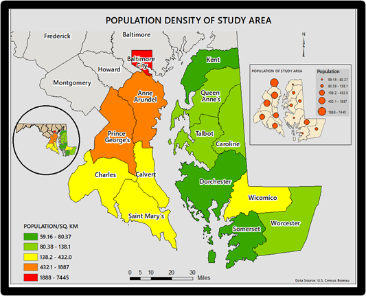 | Figure 1.1. Maryland’s Southern Region Population Density |
Accordingly, from the thermal index, the summer periods in the zone continue to be hot due to rising temperature often deemed as a major cause of fatalities, and an element fuelling ground-level ozone, a critical health risk. For that, by 2050, the usual duration of heat wave periods in Maryland, is expected to jump by over 10 to 50 days annually. Said that, this has quickened the probability of climate induced disasters to the extent that the Chesapeake Bay is listed among the most susceptible areas to climate change impacts via elevated temperature and shifts in ecological conditions. Unsurprisingly, from the average estimates in the low to upper 50°F since 1980-2022 for the region. The first 6 groups of counties (Anne Arundel, Baltimore city, Caroline, Charles, Calvert, and Dorchester) in 1980 saw visible shifts from 55.3 to 55.4°F with the 2022 temperature at 55- 58.5°F. While this represents the group’s mean values of 54.8 to 57.7 from 1980-2022, when tallied up among counties from Anne Arundel to Dorchester overtime. These counties posted 3.1 degree increases in temperature collectively. This means that over a period of 4 decades, the temperature among the counties showed steady rise. Knowing that from 2017 and 2019, the zone saw 5 dangerous rainstorms and a tropical cyclone including Hurricane Isaias in 2020. The event triggered flash floods across counties as portions of land in the Bay area came under submergence. In the process, from 1980 to 2022, the average monthly rain value rose continually. Aside from 35.3 inch-39.8 inch to over 39 inches for Anne Arundel and Talbot. In 1980-1985, over a dozen counties that averaged 42.75 inch in 1985, outpaced their neighbors [55]. Being an ecozone besieged by the rising temperature, erratic precipitation, the rising emissions of CO2 and Green House Gas concentration in the atmosphere [49]. The pace of climatic uncertainty therein, could eventually wreak more havoc. Seeing all that, surely, regional analysis of the trends in climate change in the study area, has major upsides essential in risk mitigation using the mix scale model [56-58].
2.1. Methods Used
The paper uses a mix scale approach involving descriptive statistics and secondary data connected to GIS to analyze the rising incidence of climate change and the associated issues, the exposure, and the effects of shifting weather patterns. The emphasis is on some selected counties of Maryland’s Southern region. They consist of counties starting from Anne Arundel, Baltimore city, Caroline, Charles, Calvert, and Dorchester to the others on the various axis of the state from the upper Northern area to the lower side. The spatial information for the study was obtained from numerous organizations consisting of the United States Geological Survey (USGS), the United States Department of Agriculture (USDA), the United States Department of Interior, United States General Accounting Office (GAO), and the National Hydropower Association, the World Meteorological Organization and The US Conference of Mayors. Others include Federal Emergency Management Agency, (FEMA), Maryland Department of Transportation, (MDOT), National Centers for Environmental Information, US Environmental Protection Agency (EPA) and the Maryland Commission on Climate Change.Additional geospatial data came through the National Oceanic Atmospheric Administration (NOAA), Archives of the counties in Southern Maryland, and the Government of Maryland. In addition to that, the US Census Bureau, the Maryland Online Interactive maps, and Acc Weather Inc, Nature Conservancy, Water rights group, Midwest Environmental Advocates, US Environmental Protection Agency, (EPA), The US Natural Resources Conservation Services, The County Governments of Southern Maryland, Rebuild Maryland coalition, Maryland Department of natural resources, and the Maryland Department of the Environment, also offered other information as required in the enquiry. Basically, much of the climate change related variables made up of average temperature, average rainfall time series of the region and counties, CO2 emission volumes germane to the zone collectively and the individual counties came from the repositories at the state and federal levels including National Centers for Environmental Information, Maryland Department of Planning, National Weather Center, Georgetown Climate centre, the Government of Maryland and The County Governments of Southern Maryland. On the one hand, The University of Maryland, and the other entities at the USGS, Heart of Chesapeake County Heritage Area and Preservation Maryland and the heritage area, the National Park Service, and Hurricane Sandy Disaster Relief Fund offered related information. Elsewhere Encyclopedia Britannica Inc, NASSA, United States Department of Energy, American red cross, The US Energy Information Administration (EIA) provided additional secondary data on the numbers, hydrological profile, quantities, trends, emission data and the categories as well as indicators pertaining to the shifting climate.On the other, The Southern Maryland Conservation Alliance, The Conservation Fund, Natural Resources Conservation Service, the Chesapeake Coastal Service, Maryland Department of Natural Resources, Wildlife and Heritage Service, The U.S. Fish and Wildlife Service, The Conservation Fund, the Federal Emergency Management Agency (FEMA), NOAA’s National Water Center, and the City of Worchester provided info also. Said that, the Natural Resources Defence Council, the Government Accountability Office (GAO), GAVOP and the National crop Insurance services showed essential data to complement the time series info and other valuable data on hydrological and climate change parameters. This includes indicators like Green House Gas Emissions (GHGs), the costs of liabilities and insurance premiums for inland and coastal areas from climate change induced damages by floods, drought, and other climate related info on the zone. For more data needs, regional and state, county and federal geographic identifier codes of the states were used to geo-code the info contained in the data sets. This information was processed and analyzed with basic descriptive statistics, and GIS with attention paid to the temporal-spatial trends at the state, county, and regional levels in Maryland’s Southern region. The relevant procedures consist of the two next stages listed below.
2.2. Stage 1: Identification of Variables, Data Gathering and study Design
The initial step in this research consists of the identification of variables required to analyse the extent of climate change, occurrence and impacts as manifested in the behaviour and shifts at the state, county, and regional levels from 1980 to 2022. While the elements encompass socio-economic and physical variables. The former is made up of population, population changes and the rates, population index, population per square mile, and the total population below 6 ft by county. The other components of variables in the economic information filed cover coastal premium in $, average annual premium for coastal and inland homes, coastal premiums vs inland premiums, comparable home prices in $, average flood water and delay costs, transportation fuel fees, and non-transportation fuel fees. This is followed by physical information including rainfall volume, heat index, average temperatures, average precipitation, CO2 emission rates, CO2 emission rankings, dissolved oxygen, number of CO2 emission facilities, average tidal range, Green House Gas Emissions (GHGs), emission total, regional emission total, precipitation total, rankings, percentage of emissions, and Green House Gas Emissions under business-as-usual model. The others consist of climate indicators like farm crop growing season length, number of storms, extremely hot days per year, milage of coastal lines, observed and projected temperature, 1-2 feet below sea level height, 5 feet below sea level and storm surge height, the frequency of heat waves, heat index, and the number of days under heat. These variables as mentioned earlier were derived from secondary sources made up of government documents, newsletters, and other documents from NGOs. This process was followed by the design of data matrices for socioeconomic and land use (environmental) variables covering the census periods from 1980, 1985, 1990, 1995, 2000, 2005, 2010 to 2015 and 2022. The design of spatial data for the GIS analysis required the delineation of county boundary lines within the study area as well. Since the authorized boundary lines amongst the 14 counties stayed unchanged, a common geographic identifier code was assigned to each of the area units for analytical coherency.
2.3. Stage 2: Step 2: Data Analysis and GIS Mapping
In the second stage, descriptive statistics and spatial analysis were employed to transform the original socioeconomic and ecological data into relative measures (percentages, ratios, and rates). This process generated the parameters for establishing, the extent of climate change based on the parameters, the variation in heat index, percentage and total volumes in rainfall, total temperature values and aridity intensity, the percentage of CO2 emissions, the ordinal rankings among variables. While the other dimensions that were generated embody the total emissions, number of emission sources, the percentage of CO2 emission facilities, County percentage of CO2 emission facilities, precipitation total, regional total, emission rates, monetary equivalent of insurance premiums, inland and coastal property premium ratio, population rates, and changes. Of great importance in the analysis are the use of temperature and rainfall volumes, totals and percentages across county and state levels of areas covered as well as the populations served, the frequency of flood hazards and the trends across the Maryland Southern region for each of the 14 counties through measurements and comparisons overtime. While the spatial units of analysis consist of states, regions, shorelines, and counties and the boundary and locations where inclement weather events escalated glaringly. This framework ensures the identification of change. As the graphics underscore the actual frequency and impacts, climate change induced damages, heat index and emission levels and the intensity of CO2 emissions and the trends coupled with the monetary costs of coastline insurance premium. The remaining steps involve spatial analysis and output (maps-tables-text) covering the study period, using Arc GIS 11 and SPSS 29.0. With spatial units of analysis covered in the 14 counties [Fig. 1-1.1], the study area map indicates boundary limits of the units and their geographic locations. The outputs for each county were not only mapped and compared across time, but the geographic data for the units which covered boundaries, also includes ecological data of land cover files and paper and digital maps from 1980-2022.This process helped show the spatial evolution of locations and levels of climate risks indicators, and the trends, the ensuing socio-economic and environmental impacts, ecological degradation as well as changes in other variables and factors fuelling the impacts in the region.
3. The Results
This part of the analysis focuses on temporal and spatial analysis of the climate change dangers in the study area. Using descriptive statistics there is an initial focus on the analysis of rain falls, temperature snapshot, and the chronicle of key climate events that plagued the zone in nearly four decades. The other sections, delves on the pollution audits. This is followed by the remaining portions of the section encompassing of an impact assessment, GIS mappings, and the classification of the factors fuelling changing climate in the South Florida region.
3.1. Green House Gas Emissions by Sectors 2006-2013 and 2006-2020
In looking at the breakdown of Green House Gas budget for the state, consider the trends pertaining to the events all through 2006-2013. From the actual volumes in the emissions during those periods, there were more atmospheric discharges of noxious gases in the initial four years of 2007, 2006, 2008 and 2010. Given the relative closeness of the emission values in those periods. The temporal distribution of the physical accounts consists of 109,120,613.2 TMT - 107,229,536.5 TMT and 107,167,938.9-100,126,383.9 TMT. Aside from the fact that statewide Green House Gas (GHGs) emissions in 2007 outpaced the remaining years. One clear thing in terms of the emission patterns, stems from slightly identical values in GHGs budgets between 2006 and 2008 at levels much closer to the discharged volumes in 2010. In the other remaining four years in the state’s Green House Gas budget, note that when the emission dropped further, Maryland saw its GHGs budget slide to 99,283,829.7 TMT in 2011. This was closely followed in 2009 and 2012-2013 with emission volumes of 98,489,353.1 TMT -98,284,400 TMT as it declined further by 96,799,100 in the fiscal year 2013 (Figure 2). The extended glance of the figure regarding the projected emissions of Green Houses from 2006 through 2020 offers more clues on the forms of emissions under the business-as-usual model without interventions. Unsurprisingly, as one would expect the state’s 2006-2007 GHGs emission deemed the lowest in the entire span of 14 years, went from 107,229,536.6 to 109,087,677.6 TMT. This is in deep contrast with the mid high point periods of 2017- 2018 on the graph when GHGs emission values stood at 131,476,934.6 TMT-129,350,013.6 TMT. Aside from the 2013 and 2015 GHGs emission budgets levels of (121,502,998.9 TMT -125,263,220.5 TMT) for the state of Maryland, the emission points during 2012-2016 at 119,699,499.6-127,380,964.8 TMT were also significant enough to do damage. In 2019-2020, Maryland’s emission values in the business-as-usual model surged further from 133,499,635.9 -135,679,730.3 TMT as well (Figure 2.1).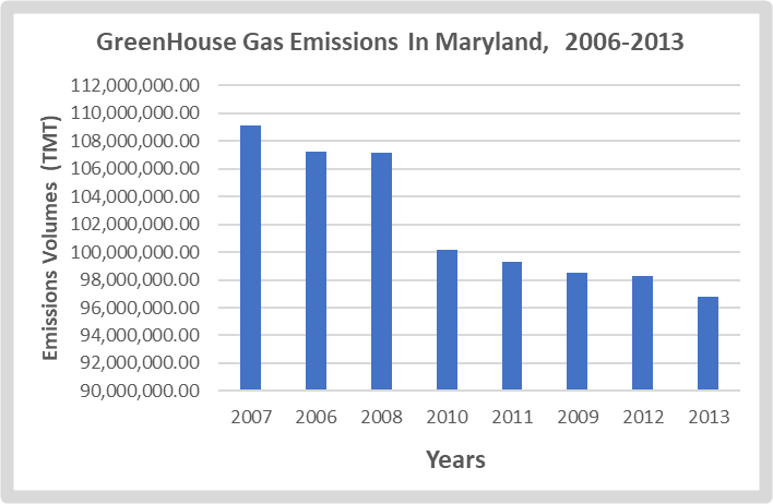 | Figure 2. Green House Gas Emission Volumes, MD 2006-2013 |
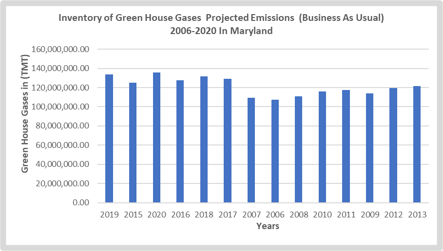 | Figure 2.1. Projected Green House Gas Emissions, MD 2006-2020 |
3.1.1. CO2 Emissions 2018
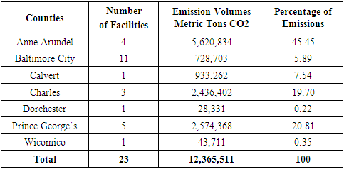
Another twist to the impacts of climate change in the study area of Southern Mary land involves the exposures to CO2 emissions emanating from different sources therein. This trend can be gleaned from the temporal distribution of CO2 emissions from several facilities operating across seven counties of the zone in 2018. The extent and form of the trends as shown on the table or the emission matrix covers the actual volumes of CO2 discharged, the facility numbers, discharged values and the respective percentages of emissions. Of the total of 23 facilities scattered around 7 counties, and responsible for 12,365,511 thousand metric tons in 2018. The county of Anne Arundel, Charales, and Prince George ‘s held about a total of 10,631,6004 TMT in 12 of the facilities, representing 85.96% of the emission volumes. Among the counties in the zone, Anne Arundel led the rest of the individual counties as the biggest emitter with 5,620,834 metric tons of CO2 at 45.45%, whereas Charles and Prince George ‘s counties emitted over 2milliom plus (2,436,402-2,574,368 Thousand Metric Tons). Just as in the second tier of counties, both Baltimore City and Calvert with combined 12 facilities accounted for 728,703-933,262 TMT of CO2 at the rates of 5.89-7.54%. Fron thereon, the duo of other lower tier counties of Dorchester and Wicomico emitted merely 28,331 -43,711 TMT. This was followed by Calvert County where about 933,262 TMT were traceable to 1 facility at the rate of 7.54% in the percentage of emissions (Table 2). Even though, at the state level in the Mid-Atlantic, a trio of neighboring states (Pennsylvania, Virginia, West Virginia) ranked 1,2,3 in CO2 emissions surpassed Maryland in all emission statistical indicators, the transboundary side can still be felt elsewhere including the study area in Southern Maryland.Table 2. CO2 Emissions Sources in Counties In the Study Area 2018
 |
| |
|
3.1.2. The Temperature Patterns Regional and County Levels 1980-2022
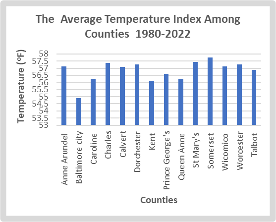
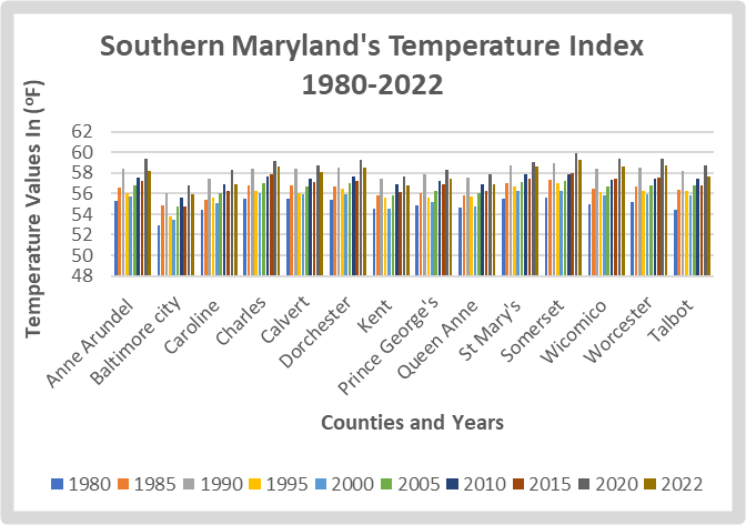
In the face of mounting shifts in climate parameters, note that the mean regional temperature values from 1980 to 2022 were in the low, mid, and upper 50-degree Fahrenheit with 2020 the highest (Figure 2.2). For that, the first 6 group of counties consisting of Anne Arundel, Baltimore city, Caroline, Charles, Calvert, and Dorchester in 1980 all saw visible shifts from 55.3, 52.9, 54.4, to 55.5 to 55.4 degrees coupled with the temperature readings in 2022 of 58.2, 55.9, 56.9 to 58.6, 58.1 to 58.5 degrees. This represents a group average of 54.8 to 57.7 from 1980-2022, when tallied up among these counties from Anne Arundel to Dorchester over time. Taking a cue out of the profile, the said counties collectively experienced at least 3.1 degree increases in temperature. Elsewhere at Kent, Prince George’s, Queen Anne, St Mary, Somerset, and Wicomico counties in 1980, the atmospheric conditions held steady in the mid 50 degrees (54.5, 54.9, 54.6, 55.5, 55.6, 55.0) at that time. When added up closely again based on the values for 2022 (of 56.8, 57.5, 56.9, 58.6, 59.3-to-58.6-degree Fahrenheit) one sees varying averages of 55 degrees in 1980 and slight jump to 57.9 degrees in 2022. This means that over a period of four decades plus, the temperature among the counties continued to show steady rise. Looking at the temporal snapshot of remaining duo of the counties made up of Worcester and Talbot throughout 1980 to 2020. The modulation in group temperatures (55.2-54.4 to 58.7-57.7) for 1980 and 2022 respectively, yielded averages of 54.8-to-58.2-degree Fahrenheit with increases of over 4 degrees over a span of 4 decades (Figure 2.3). Another dimension to the county level temporal average profile involves the sum of all temperature from 1980-2022. This offers a better insight into the actual individual county temperature total. As mentioned earlier, and with most of these places averaging temperature levels of high and mid-50s in degree Fahrenheit. It came as no surprise that temperature distribution between 1980-2022 among the counties indicates 8 (Anne Arundel, Charles, Calvert, Dorchester, St Mary, Somerset, Wicomico, and Worcester) of the 14 had temperature levels of over 57 degrees Fahrenheit. While this is followed by another quintet of counties (Caroline, Kent, Prince George’s, Queen Anne, and Talbot) classified under the 56 degrees plus category, only Baltimore city accounted for 54.9-degree temperature levels when contrasted with the others at 54.9 -56-degree average threshold in the listings. Having come this far at the regional level, see that out of the initial slow build up in recorded temperatures in the decades of the 1980s (1980-1985), the variability went from 54.90 -56.34 degrees Fahrenheit. By the 1990s, the region saw further fluctuations in temperature measured in the order of 58.07 to 55.98 between 1990 to 1995. Notwithstanding the initial stability in the 2000s at 55.47 -56.50-degree Fahrenheit in 2000 to 2005. The study area still never left one in doubt on its reputation as the locus of fluctuating temperatures (of 57.28 -56.94 to 58.73 -57.87) in almost 2 decades from 2010 to 2020 (Figure 2.4).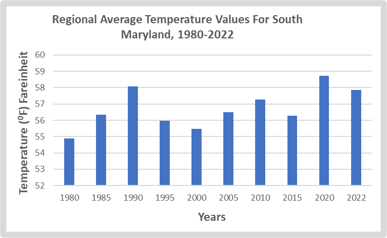 | Figure 2.2. Regional Average Temperature Values South MD 1980-2022 |
 | Figure 2.3. The Average County Temperature Index South MD 1980-2022 |
 | Figure 2.4. The Average Temperature Index South MD 1980-2022 |
3.1.3. The Rainfall Levels 1980-2022
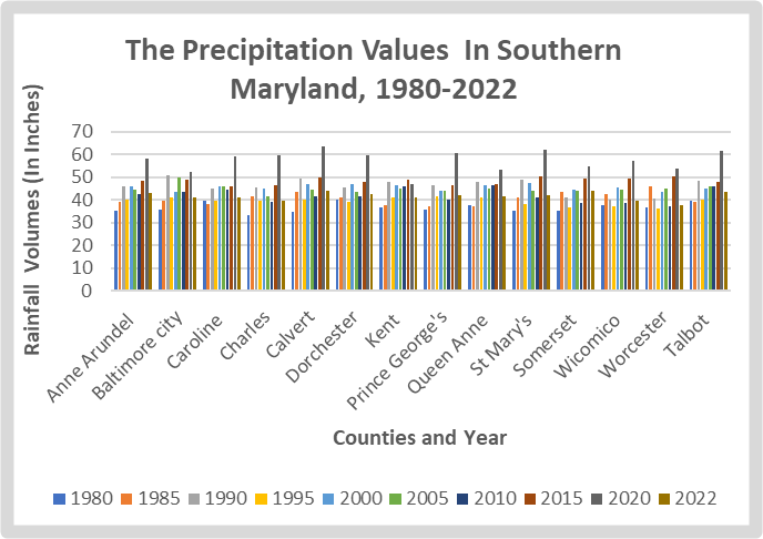
Just as the monthly rainfall averages in the region surged yearly (Figure 2.5). Among the counties from 1980 to 2022, precipitation rose much of the time over a period of 40 years across the board. Aside from precipitation values estimated mostly in the 35.3 inches – to 39.8 inches category to over 39 inches from Anne Arundel and Talbot (Figure 2.6). In the first years of 1980-1985, over a dozen group of counties (Charles, Calvert, Dorchester and the other quartet St Mary, Somerset, Wicomico, and Worcester) who posted group average values of 42.75 in 1985, outpaced their neighbors. Along those lines, both county and regional average and totals not only reached 57.35- 803 inches all year round in 2020. Among the counties, Calvert, St Mary, Prince George’s, and Talbot accounted for over 60 inches (63.7, 62.0 to 61.5 -60.8 inches) far ahead of the other areas (Figure 2.7). In other words, the precipitation level in 2020 seems to have surpassed the other years in the hydrological calendar of Maryland’s Southern region (Figure 2.7). Against that background, even the heavy surges in rain falls based on decadal averages and totals of 39.4 – 42.52, in 1990, and 2022 still paled in comparison to the 2020 season. The same thing goes for 2005 through 2015 during which all counties from Anne Arundel to others soaked in over 46 inches and above except for 50 inches and above during 2015 in a trio of Southern counties most notably Calvert, St Mary, and Worcester. In going back to the most recent year of 2022, the temporal profile in place for the counties and the whole region estimated mostly at the 41-to-62-inch average levels and a total of 582. 99 still fell short of the 2020 record.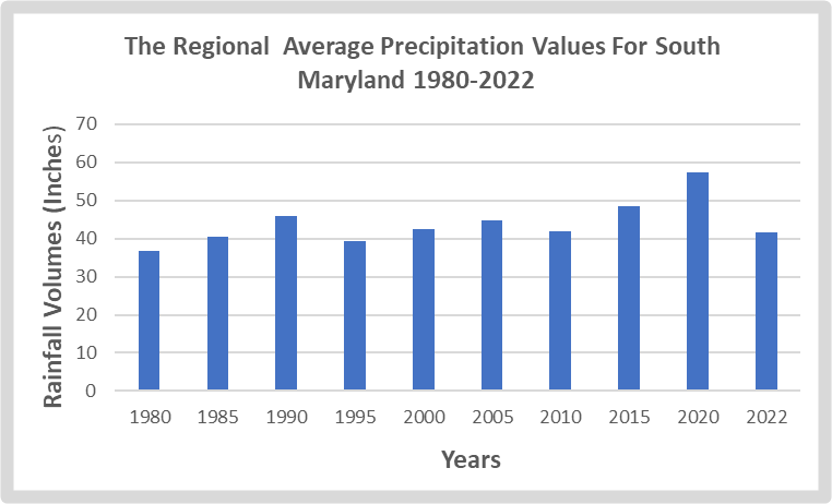 | Figure 2.5. Regional Average Precipitation Values, South MD 1980-2022 |
 | Figure 2.6. Regional Average Precipitation Values, South MD 1980-2022 |
 | Figure 2.7. The County Rainfall Volumes, South MD 1980-2022 |
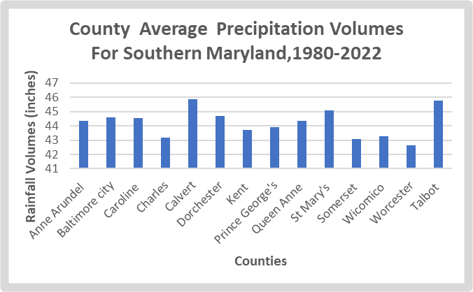
In as much as precipitation levels show some visible drops based on the info gleaned from the table, the counties of Calvert, Talbot, Somerset and St Mary and Prince George’s and Anne Arundel with values of 44.1 inches, 43.9, 43.6 inches to 42 inches plus. Anne Arundel and Dorchester still topped the list when compared to Baltimore city, Caroline, and Queen Anne where precipitation stood at 41 inches plus. The remaining counties of Wicomico Worchester and Charles in the zone saw their precipitation levels vacillate between 39.5- 37.6 inches to 39.6 inches at levels below the other counties in 2022. When it comes to the detailed outline of the precipitation breakdown among the counties between 1980-2022, the trio of counties as headlined by Calvert, Talbot, and St Mary had more rains. This stems from the totals and averages measured at 458.9 to 45.89, and 457. 3 -45.75 followed by St Mary at 550.9 – 45.09 inches. The precipitation volumes as displayed on the tables remained higher than the levels in the same period for a quartet of counties Anne Arundel, Baltimore City, Caroline, Dorchester, and Queen Anne where the ratio of the sum and averages consisted of 443.6 44.36, 446.19-, 44.61 and 445.4 inches to 44.54 inches from 1980 through 2022. In that order, the counties of Charles, Kent, Prince Georges, Wicomico, and Somerset at identical values of 431.8- 43.18, 437- 43.7 inches, and 439- 43.9, 432.6-43.26 to 430.7-43.07 rounded out the group three level of counties. These places were battered by notable volumes of rain over the years until it faded at Worcester County by 426 inches to 42.6 inches. The regional precipitation highlight also covers a mix of intensity, slowdowns, and surge in accelerated downpours over time. To the effect, beginning in 1980-1985, mild occurrences in downpours, reached average and total volumes of 36.67 inches to 513.5 and 40.52 inches -567.4 inches. In the 1990s, came brief surge of rainfall values measured at 45.88-643.839.4-551.6, while more downpours peaked up further steam with mean and overall tallies of 42.52-637.3 to 44.81-627.4 by 2000-2005. In the ensuing years of 2010-2015, the pace of rain fall changed further by 41.87-586.3 to 48.37-677.2 inches. This uncertainty surrounding unpredictable rainfall patterns emerged again further in 2020 through 2022 based on average and total values of 57.35 inches to 803 inches and 41.62-582.99 respectively.
3.2. Impact Assessment
Looking at the recurrent risks from climate change in the South Maryland region. The built and natural environment in the form of community neighbourhoods, petroleum infrastructure and fragile ecosystem were at the receiving end of sustained and future impacts of varying proportions.
3.2.1. Economic Impacts
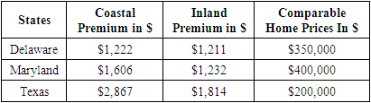
Considering the impacts of shifts in climate it is evident that heavy floods from storms can interrupt journeys and trigger dangers, while accelerating economic losses. In fact, the flooding of state highways in Maryland is responsible for several days of road traffic interruptions yearly, at an of average of 1,582 hours—or 66 days—per annum. In such settings, many of the traffic lane closures responsible for interruptions persisted under a period of 4years as 16% of every disruption went on for over 12 hours. Furthermore, looking at the average home price of $400,000 in Maryland, house owners remain vulnerable to escalations in the price of repairs from damages inflicted by natural disaster on homes situated along low lying points and counties in the study area. With the breakdown of the comparative insurance premium costs for both coastal and inland homes in counties and cities for Maryland at $1,606 to $1,232 (Table 2.1). The costs for inland and coastal properties exemplify the volatility of liability pricing during unexpected disasters. In as much as the zone is besieged by liabilities from recurrent floods. The disruptions not only affect over 480,000 citizens yearly, but the delays can also translate into monetary losses as well. Seeing that the cost of missed work time and suspended supplies at about $15 million annually in Maryland, reached over $230 million in a span of 15 years due to climate change. As a result, every flood event accelerated the mean value of around $80,000 in user delay costs. Nonetheless, flooding also has the capacity to hamper sources of income and survival across neighborhoods and counties in any period in the year if besieged by stressors, and drivers of key disasters. When these incidents occur with greater recurrency and intensity minimizing traffic circulation, by flooding roads, and destroying amenities, the ensuing costs and liabilities escalate alarmingly. Table 2.1. Average Annual Premium of Coastal vs Inland Homes For Comparable Policies
 |
| |
|
3.2.2. Social and Demographics
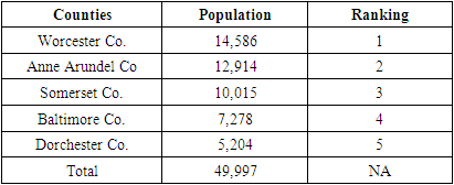
Added to that, in as much as the typical roadway floods costs the state of Maryland about tens of thousands of dollars in travel costs and business delays from 2006 to 2020. Understand that it is occurring in a setting where a significant number of the properties are at a high risk of the dangers of inundation along the counties. In fact, during the fiscal year 2010, close to a total of 50,000 people resided in places deemed below 6 ft. Besides the demographic and ethnic breakdown of those threatened by coastal hazards because of climate change at 7,343, 64,149, to 2,163 for African Americans, Whites, and Latinos among the population. The vulnerability rankings of those at-risk counties in the year 2010, reveals the susceptibility of a trio of areas (Worcester, Anne Arundel County and Somerset County). Seeing that these places are besieged by greater exposures to spots below 6 feet with populations estimates in the tens of thousands starting at 14,586, 12,914 - 10,015 in 2010. The same risks levels extend further to 2 other counties (Baltimore County and Dorchester County) ranked 4 and 5 under the thresholds and listed on the critical hazard prone areas of 6ft below the sea level with vulnerable populations of 7,278 -5,204 (Table 2.2). Table 2.2. Total Population Below 6 ft in Maryland 2010
 |
| |
|
3.2.3. Physical and Ecological Impacts
From the enquiry, Southern Maryland saw recurrent climatic shifts, widespread risk exposures through periodic damages to the ecosystem, along with fiscal losses in some sectors of the economy. With the impacts manifested through pollution, ecological decline, and degradation. It can no longer be ignored, that climate change is by now, having a dreadful effect on Maryland’s coastal communities. Being a place where thousands of citizens reside near to land area on 3,000 miles of coastline where nearly ¾ of the populace reside and work. The threat level from unprecedented devastation looms larger continually. Considering the pace at which nuisance flooding in Annapolis, Maryland from March 7, 2018, occurred through rising tides. From 1960 to 2020, tidal flooding days per year has really intensified overwhelmingly from under 5 days between 1960-1990s until it reached the five-day level in 1999. In the following years in 2009, the increasing frequency in flood events surged further to 6-7 days. Over time, from 2010-2019, the occurrence of tidal flooding moves from 10-13 until a rise of 15 -18 in the year 2020 along the Annapolis area. As a measure of the gravity of the situation, the number of frost days in the Chesapeake area of Ann Arundel County has declined drastically between 1980-2010 from 1970 levels to current levels of merely under or below 80-70 days. Just as the average diurnal tidal range at active gauge stations in Maryland has arisen among cities in the study area, coastal wetlands in the zone have also come under huge threats. In the process, under a decade of coastal flooding days, Annapolis saw an overall total floods of 394 from 2005-2014 with ¾ of all that from anthropocentric sources. Elsewhere, The Chesapeake Bay remains one of the most vulnerable regions in the nation to the effects of climate change. Some of these effects—including rising water temperatures and surging sea levels—have already been observed, and the region is expected to experience further shifts in environmental conditions. Additionally, over the past century, the Bay waters have risen to about one foot, and are predicted to rise another 1.3 to 5.2 feet over the next 100 years. This is faster than the global average because the land around the Bay is sinking rapidly through a process called subsidence.
3.3. GIS Mapping and Spatial Analysis
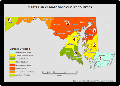
The GIS analysis covers the visual expression of geographic patterns highlighting various indicators describing climate shift dangers in Maryland’s Southern region based on the Maryland Environmental Management Areas (MEMA) and climate divisions. Accordingly, the initial risk parameters as captured in the map encompasses rainfall intensity and changing temperatures over the periods 1980 through 2022 across the spots on the maps representing multiplicity of counties in the region from Baltimore city to Worcester. Additional elements shown in the map consists of information in the legend boxes pertaining to sea level rise, hurricane disaster categories at various scales, flood hazards and sea level rise thresholds. Focusing on the dilemma of the disasters in the region across time, the data as manifested by the GIS mapping on the dimensions, affirm the evolving forms in space. The capacity in pinpointing the geographic pathways of the patterns in a GIS environment as analytical device, provides opportunities in carrying out climate change impact assessment on Maryland’s Southern region.Considering the risks posed to the state of Maryland, the geospatial analysis of the annual average rainfall from 1980 -2020 in Southern Maryland, shows possibilities exists to unravel the climatic uncertainties. From the info on the map differentiated by colors and scales of green, red/orange, and yellow highlighted across regional lines. Out of these patterns emerges gradual spread in light and dark yellow colors in the lower South as represented in Charles and St Mary’s coupled with the Southeastern shorelines in Worcester County in deep yellow. Considering that these spatial patterns in rainfall, were prominent in the left and far right lower sides of the map on the scales of 45.09 to 43.18 inches to 42.6 inches between 1980-2020. The next wave of spatial evolution mostly in different shades of green with heavy concentration in the north central and Northeastern axis, and the central portions of Southeastern shores erupted all the way from Baltimore city, Queen Anne, Caroline, Wicomico, Dorchester, and Somerset with average rainfalls levels of 43.06, 44.7 inches, 43.26 inches to 44.61, 44.37 inches. Among the areas denoted, out of the red and orange colors, comes Kent and Talbot with rainfall average values of 43.9-45.75 inches slightly similar in volumes at 45.89 inches -44.36 to 43.7 in neighbouring counties of Anne Arundel, Calvert, and Prince George’s all in the upper and lower tip of the state’s county climate divisions in over 4 decades from 1980-2022 (Figure 3). 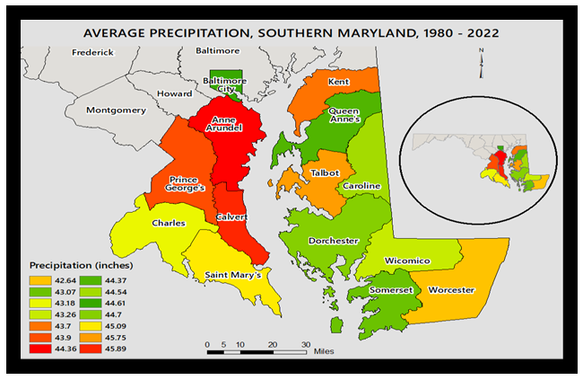 | Figure 3. Average Precipitation Southern Maryland 1980-2022 |
With much of the areas that came under a spell of the highest precipitation levels during the 1980 chiefly situated along the right side of the map mostly in the green shades of thick to light coupled with orange colors across the northeast and lower south shore axis. This is where the counties of Dorchester, Talbot and Caroline seems to have been at the receiving end of greater intensity of the average monthly rain estimated 38.9 inches to 39.8 inches throughout the period 1980 while Queen Anne and Wicomico on the other end both averaged 37.8 inches. Further along that order, precipitation levels for Kent and Worcester each reached 36.5 inches to 36.9 inches during the same time. Additionally, the left end of the map legend also highlights a mix of mostly yellow, red, and orange symbols gathered in space from upper northwest to the south corner. In these group of counties, under which the volumes in rain in the initial quartet reached the plus 35inch mark, in the mean values in more than 4 decades, Baltimore city in the upper north leads its neighbors in that category by 35.6 inches right in the vicinity of Prince George’s at 35.5 inches in rain volumes as 3 other counties (Anne Arundel, Somerset and St Mary) stayed firm at 35.3inches to 35.2 inches. From the evolving shifts in rainfall intensity, both Charles and Calvert County also saw heavy rains but at levels slightly lower than the former at 33.3 inches to 34.8 inches (Figure 3.1). 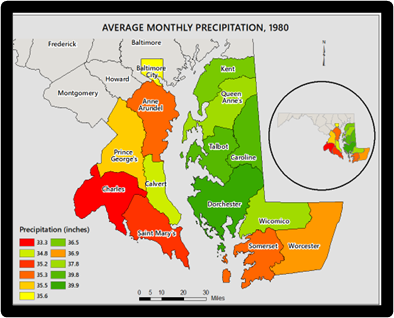 | Figure 3.1. Average Monthly Precipitation Southern Maryland 1980 |
The distribution of average precipitation patterns in the 2020 period, indicates the areas with heaviest levels on the right side with Calvert, Wicomico, St Mary’s, and Worcester County above the rest at 63.7-62inches and 61.5 inches. Within the same period in the season 2020, emerges more dispersions in heavy precipitation into other points in space where Prince George’s and Charles appeared under heavy precipitation levels of 60.8 inches -59.9 inches. From there emerges another trio of counties, most notably Dorchester, Caroline, and Ann Arundel with precipitation values of 59.7-59 inches to 58.3 inches followed by Somerset County at 54.6 inches. In the next batch of areas under the purview of average monthly in the lower end of the scale, starts Kent, Baltimore city, Queen Anne, and Talbot under heavy precipitations values of 47.1 inches, -52.3 inches, 53.3 -53.8 inches (Figure 3.2). The summary of the average monthly rainfall in 2022, being the most current, provides a major contrast from the previous. As such, the geographic pattern in the spread reflects color lines of mostly red /orange, green and yellow. Since the numeric value of precipitation classifications falls under three segments, the initial 5 group of counties from the upper northeast and lower Southeast side comprising of Caroline, Kent, Worcester, Anne Arundel, and Dorchester took the center stage, with rainfall values of 44.1-43.9 inches, 43.6 to 42.9-42.5 inches deemed above. In the same year, emerges further shifts in the dispersion of rainfall values towards the left corner of the map as another quartet of counties (St Mary’s, Prince George’s, Queen Anne, and Calvert at 42.3, 42, 41.6 to 41.3 inches) manifest the variability in precipitation. Looking at the other dimensions in the average monthly precipitation, note the dominant presence of places identified by clusters of mostly orange, red, and yellow. The said points and rain fall values in space encompasses 41.19 -40.9inches to 39.6 inches for Baltimore city, Somerset, Charles, whereas Wicomico and Talbot were soaked by 37.6 inches as part of their monthly average precipitation (Figure 3.3). 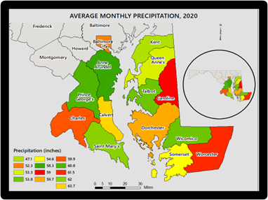 | Figure 3.2. Average Monthly Precipitation Southern Maryland 2020 |
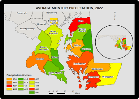 | Figure 3.3. Average Monthly Precipitation Southern Maryland 2022 |
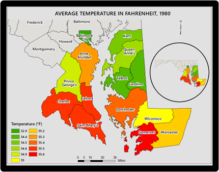
With concerns over changing temperature and the threats of global warming. The summary of the info from 1980-2022 in the map legends contrasted in various colors indicates, seem mostly separated by a ratio of over 57°F to 54°F plus. From the listings in space, many of the counties averaging 57°F in temperature extend far deeper onto the upper and lower sides beginning from central shore and upper southern shore of the maps. From there comes avalanche surges in temperature beginning which resulted in 57.13°F for Arundel, Wicomico County, followed by 57.45°F at St Mary’s as Dorchester and Somerset became fully trapped in the higher end of the temperature scale at 57.35 -57.7°F correspondingly. Elsewhere, see Queen Anne and Calvert immersions into heat axis by some measure at 57.09°F. The couple of counties listed under the 56°F category stretched through Talbot, Kent, Caroline, Prince George’s with temperatures deemed in similar ranges in the mix at 56.87°F to 56.12°F and 56.25°F-56.59°F. In the zone, Baltimore city at 54.09°F stood out as the outlier below the counties in the greater region of the study area (Figure 3.4). The temperature side of the analogy in 1980 from the scale of 52.9 -55.6°F for the counties in the study area appears evenly matched on the spots in space. These points are covered under red/orange shades concentrated mostly on the right part of the legend box and the green /yellow scales loaded on the left side of the box. However, the geographic dispersion of the temperature values for the period 1980, reveals a Northeast and lower southwest divide with slight crossovers. Per se, the counties of Somerset in lower south, St Mary’s, Charles, and Calvert experienced temperature levels of the high scales (55.6°F, 55.5°F, to 55.4°F) as Dorchester, Anne Arundel and Worcester saw slightly identical temperature levels of 55.3°F to 55.2°F. On the other side of the temperature scale in 1980, Wicomico and Prince George’s, Queen Anne, and Kent came under humidity levels of 55°F, 54.9°F to 54.6°F with the temperature shifts in the last three counties (Caroline, Talbot, and Baltimore city) vacillating from 54.5°F, 54.4°F to 52.9°F (Figure 3.5). From a closer look on the study area’s temperature patterns, one notices an interesting occurrence where the set averages of 59°F plus manifested in 5 places in the 2020 period apart from the others to some degree. This sudden surge to 59°F as the map indicates, starts with the situation in Somerset, Wicomico, and Anne Arundel counties where temperatures of elevated scales at almost 60°F (59.9-59.4) reached all-time highs. The uptick in temperature scales of 59.3°F, 59.2°F, to 59.1°F continued further at Dorchester, Charles, Calvert, Worcester, and Talbot. The second category of temperature surge on the map provides an outline of identical scales of 58.8°F, 58.3°F, 57.9°F to 57.7-56.8°F in the counties of Calvert, Caroline, Prince George’s, Queen Anne until Kent, Anne Arundel, and Baltimore finished at 56.8°F -55.9°F at the other end of the scale (Figure 3.6).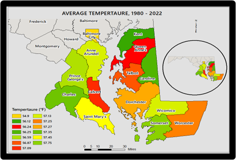 | Figure 3.4. Average Temperature 1980-2022 |
 | Figure 3.5. Average Temperature 1980 |
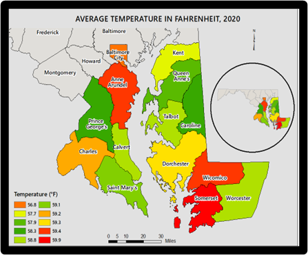 | Figure 3.6. Average Temperature 2020 |
In the 2022 portion of the averge temperature summaries for the study area, Worcester and Talbot, Wicomico and St Mary’s, Charles, and Dolchester and Anne Arundel came under hotness levels of 59.3°F, 58.7°F, 58.6°F, 58.5°F to 58.2°F. Under the next clssifications in temperature in the 2022 season, Calvert, Somerset and Prince Gorge’s emerged as the first set of three counties drenched by temperature scales of 58.1°F, 57.7°F, to 57.5°F. After that comes further spread of the temprature levels into Queen Anne, Caroline to Baltimore city in the North and Talbot in the North east central and lower South (Figure 3.7). In light of the vulnerability of the study area to the threats of seal level rise, the risks remain real across the counties. From the map legends, denoted in blue and red colors of 2ft-5ft in sea level exposures and emergent patterns along the lower side. The region faces two pronged risks out of the scenarios highlighted on the spots in space where the rise in the 2 ft category in blue appears prominent and the 5ft projected spread, deemed likely. In as much as the parts denoted in blue stretches acrosss spots on the upper and lower shores. The pockets of counties considered at risk of eventual rising of the sea level under the 2 ft and 5 ft thresholds extends to Caroline and Dorchester. Elsewhere, the dimensions of sea level rise in the 5 ft category apeared more vissiblly towards the middle and southern portions, with a mix of both 2-5 feet sea level in place (Figure 3.8). This can excerbate the liabilities to the detriment of communities in the at risk areas. Furthermore, the 2020 versions of the storm surge hazzard levels, cover clusters of eventual landing spots denoted in green and yellow surge levels at the different scales of 1-3, 4-5ft, 6-8 to 9-10 ft and the above, vissible in the lower south east corner of the map. While all these are reflctive of the areas under the jurisdictions of MEMA in the zone, they really reflect the actual climate divisions as well (Figure 3.9-3.11).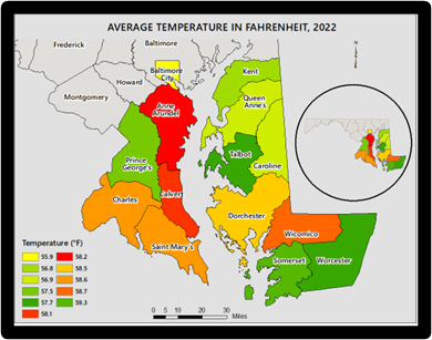 | Figure 3.7. Average Temperature 2022 |
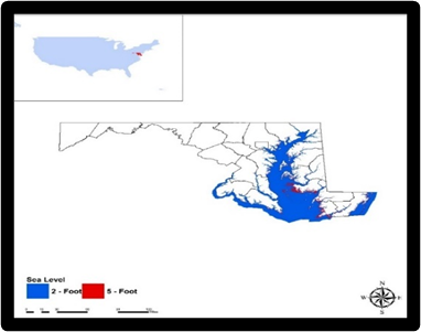 | Figure 3.8. Sea Level Rise |
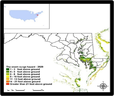 | Figure 3.9. The Storm Surge Hazzard 2020 |
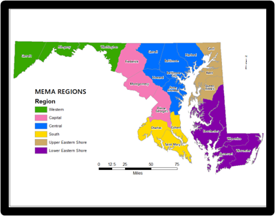 | Figure 3.10. Maryland’s Emergency Management Agency (MEMA) Regions |
 | Figure 3.11. Maryland’s Climate Divisions By County |
3.4. Factors Responsible for Climate Change
Regarding the factors triggering changing climate in Maryland’s Southern region off the US mid Atlantic zone, from all indications, they do not happen in isolation. On the one hand they emanate from forces anchored in population shifts and obsession with urban growth as well as economic and fiscal benefits deeply rooted in socio-economic, policy indicators. On the other hand, they risk exposures to changing climate emanate from physical or environmental factors These elements are examined fully in the following paragraphs.
3.4.1. Population, Urbanization/ Uncontrolled Growth
From the scale of change in the zone, the teeming population and uncontrolled growth level in Southern Maryland are all seemingly connected. While the study area’s population went from 2010-2020 at 2,710,594- 2,867,437 to 2,854, 499 on a rate of 5.04%. Among the largest counties in place, Prince George’s maintained large population figures of 863,420, 967,201, to 955,306 and posted the highest gains of 9.61% from 2010 to 2021. The third largest county Anne Arundel with big population numbers of 537,656, 588,261, 590,336 grew by 8.92% between 2010, 2020 through 2021. Another county Baltimore city opened with 620,961 in population figures in 2010, until it went to 585,708 -576,498 in the subsequent years of 2020 and 2021. The surge in population growth rates and the demand for new infrastructures based on the issuance of new building permits as catalysts for development, fuels the rapid pace of urbanization known to accelerate GHGs emission and risks to communities. This coincides with the discharge of GHGs statewide from sectors tied to households that are indicative of the trajectory of growth patterns like waste management, fossil fuel industry and transportation with emission levels estimated at 9.29 MMT, 4.03 MMT to 33.9 MMT. Considering the correlation between population growth rates and growing propensity to GHGs emission exposures, the population, trends in big urban centres and resultant surge in emission cannot be ruled out as major forces driving the proliferation of climate change chaos in the Southern Maryland. Moreso, the dredging of coastal wetlands to make way for urbanization and the attendant deforestation leads to the loss of emission sinks and formation of urban heat Island contributing to the warming of the atmosphere and elevated temperature. Granted the concerns over deforestation, and the disturbance of forest landscapes at meagre rates in the past 10 years. The urban growth continues to precipitate disappearance of woodlots statewide, particularly along the fast-growing border areas near to Washington, DC. Starting with more than 19,000 acre declines in forests land areas between 2013 to 2018, the state saw losses of 118,000 acres from 1999 through 2019, at a yearly level of declines of 6000 acres. The six counties at the centre of the losses most notably, Prince George’s, Montgomery, Anne Arundel, Charles, Calvert, and Baltimore were responsible for about 70% of entire tree cover and forest losses, with serious dangers to stability of the ecosystem in ways that fuel climate change.
3.4.2. Economic and Fiscal Benefits
The economic benefits presented from fossil fuel dependent sectors of the economy like households, industry, power utility companies, the farming sector, and the use of automobiles on the road and commercial sector are all implicated in climate change challenges. Since the tax revenue base generated from these sectors are part of the economic engine sparking the study area. But they leave in their wake climate change risks that are indicative of the role of these variables in unleashing ecosystem liabilities. This makes it very difficult to ignore in the search for factors given the place of oil and gas use and energy sector. As such, no matter the proactive nature of policy and programs towards mitigation, current economic incentives in place allows knowingly and unknowingly indulgence in practices that put communities in harm’s way. The prospects of booming development of new settlements together with business parks require clients in adjoining new neighbour hoods and school districts to thrive, commute and generate huge revenue. This makes it hard to scale back on production and new infrastructure design to spark economic expansion and the surge in carbon footprints in sectors heavily tied to the emission of Green House Gas. Thus in 2012, Maryland took in $70.55, billion dollars in real estate and rental as part of real value added in the GDP and not to talk of the $50.22 billion in value added GDP from manufacturing known for heavy duty machinery use that is energy intensive. This is in addition to transportation, warehousing, and utilities operation with the capacity to impede any Best Management Practices towards mitigation. The fact that common erratic patterns germane to cyclic atmospheric temperature across the Northeast, increases energy requirements for heating and cooling, in the winter season gulps up more power loads. For that, the electric power sector ranks high as the top natural gas user among other sectors, so in the fiscal year 2021, the sector used up an unprecedented amount of hydrocarbon. In the case of the state of Maryland alone, based open data access for the periods 2006, 2011, and 2020, sectors like electricity, residential and commercial, industrial, and transportation gulped vast volumes of fuel. In that light, both industry and fossil fuel use, rank high as major sources of Green House Gas emissions. During the fiscal year in question, the breakdown was in the order of 29.77-18.32 to 13,64, 8.37, to 7.26, 4.89 MMT for transportation, electricity use, residential and commercial, industrial, and waste management, and the fossil fuel industry.
3.4.3. Ineffective Policy
The state of Maryland is not only very proactive in matters pertaining to the mitigation of environmental risks, but it prides itself as a pacesetter in various aspects of planning including, the institutional, historical and administrative dimensions of land use far ahead of its neighbours. Additionally, granted the efforts including the promulgation of state policies, local and county initiatives to minimize the gravity of climate change. The problems persist because of the ad-hoc nature of responses to environmental emergencies coupled with the transboundary and global nature of the challenges. In the face of all these, given the fact that climate change does not respect ecological and administrative boundaries of states and counties, complicates the matters in ways that render well thought out policy implementation ineffectual. In the process, mitigation measures can look good on paper, but the sudden way climate change induced disasters erupt, regardless of the presence of advance early warning systems, makes responses panicky, hard to coordinate and synchronise sequentially. Because intervention measures are still rooted in templates reliant solely on reactive mode, the study area is not immune from being at the receiving end. In such setting, the transboundary, global, and regional attributes of most stressors and climate parameters like GHGs and CO2 and warming of air besieging the zone when difficult to control, can impede policy implementation, hence the current challenges in the study area despite having the capacity to adjust towards mitigation. Out of the hesitancy towards mitigation in public discourse where some downplay the gravity of climate change. The recourse to contradictory statements on the climate change puts places deemed in danger at the mercy of sceptics in settings where denial of climate change risks by elected officials are reinforced by those clamouring to defund the EPA. This is happening in a way that keeps the counties, state, and the nation unready for climate change induced disaster mitigation. Such practices are at odds with safe environment.
3.4.4. Environment and Climatic Forces
Environmental factors are among key forces fuelling the shifting climate in the study area. The location of the study area in one of the wettest areas in the Mid Atlantic known for the rising pace of hurricanes amidst the melting of Arctic Ice or polar ice caps over the years by global warming constitutes a big exposure detrimental to the ecosystem. Accordingly, between 2006 to 2013, the state of Maryland’s Green House Gas emissions reached very high levels of 816,501,155.30 TMT in noxious substances at an average of 102,062,644.21 TMT. At the same time, the states, Green House Gas levels surged in 2007,2006 and 2008 to unprecedented volumes far ahead of the other years under analysis. Additionally, CO2 emissions have shown notable increase with burning of fuels such as coal and gasoline, thereby accelerating the occurrence of and dispersal of heat waves in the atmosphere considering the pace of rising temperature. During the fiscal year 2018, CO2 emissions total from facilities in the zone were responsible for the release of 12,365,611 TMT based on the average of 1,766,516 TMT. Certainly, the concentration of CO2 in the atmosphere in such settings and rainfall events are also fuelling the increased pace of sea-level rise within the study area’s shorelines. Having endured countless storms within the cities and counties, in the years 2015 and 2020, the Southern region of Maryland posted record breaking levels (48.37-57.35 inches) under rainiest days calendar in rainfall events regionwide. Seeing the vulnerability to violent rainstorms and the nearness to the Atlantic Ocean, the region’s mean yearly rainfall and temperature (43.90 inches and 56.8°F) from 1980 through 2022, provides insights into the shifting climatic factors in the region.
4. Discussions
Seeing that state Maryland still stands out as a pacesetter in various dimensions of ecological mitigation than the others, but this has not translated into any form of immunity to common exposures to climate change dangers despite the capacities of Maryland. From the current records of inclement weather events in the Mid Atlantic zone. In the past years, Maryland continues to experience sudden shifts in climatic patterns of warmer and raining conditions reflective of repeated barrages from hazardous weather situations. In the process, while temperatures have surged to 2.5°F, and the frequency of extreme warm spells soaring. The same state that boosts of some of the most booming farming operations and a promising economy strongly dependent on a secure ecosystem, stands currently as the epicentre besieged by seemingly different forms of extreme climatic events along the coast. Accordingly, the lower side of Maryland has experienced ample scale of climate change induced dangers like ice storms, floodings and elevated temperature. Since all these are resulting in widespread damage to society, economy, and the surrounding ecosystem, amidst the vulnerability of many sectors. The applications of Mix scale methods anchored in the integration of geospatial device of GIS served vital purpose. From the analysis as carried in this enquiry, it stands clear that the South Maryland region, and the areas and towns in the zone share essential capacities shaped by the thriving landscape, diverse environment, and economic opportunity amid growing risks from changing climate. These notwithstanding, the communities and counties in the region show immense fiscal capacities, sustained by obvious existence of agricultural croplands, network of state, national, regional, and urban and private sector and industrial infrastructures in energy and utilities run by power providers and others. Added to that, is the pace at which vast structure of urbanizing areas with population concentration of new development activities are encroaching into spots characterized by green spaces. This is not only resulting in wood land clearance as manifested with the incidence of forest disturbance, but it also raises questions about commitment in conserving the much-needed emission sinks as one would have expected. Such contradictions in the efforts towards mitigation of global warming in places already at risk, can impede any gains made in minimizing rising temperature and escalation of carbon footprints through the emissions of CO2 and the production of Green House Gaes among electric and power utility sector and others. This can be gleaned from the emission budgets over the various years from 2013-2018 and 2006 through 2020. Furthermore, in keeping with the obsession with town growth, the study areas like in other places experienced the conversions of wetlands to pave way for development. Because what transpired in all these years requires the draining of coastal marsh ecosystem, that were supposed to be performing natural functions as reservoirs in the containment of climate change induced floods. This is not only occurring in a setting where Dorchester’s tidal marshes are at the epicenter of shifting climate’s effect on the Chesapeake Bay. But there are still fears pertaining to fresh sediments flow out of floods as the anticipated destruction of tidal marsh amounts to exposures to further risks for the zone’s apparently fragile urban environment. The fact that the vast capacities in the region are deeply spread along the coastal grasslands near to the Chesapeake Bay side. The ecosystem diversity therein, remains constantly threatened by the intensity of stressors of climate change induced disasters. This involved the way unprecedented city development in a quartet of large urban counties (Prince George’s, Anne Arundel, Charles, and Calvert) are listed among areas responsible for the disappearance of 6000 acres yearly and 70% of mostly forest losses between 2018-2019 along the Washington DC suburbs. Given the enormous concentration of hundreds of thousands of people in the major urban centres along the low-lying South Maryland’s coastlines. While these places extend deeper into the Anne Arundel corridors near to the places in the Bay presently endangered by projected sea level rise. Undoubtedly, the extensive proclivity to changing climate risks, will be felt among the residents, their homes, and populations in the zone. From the pressures triggered by the decades in coastal flooding days, Annapolis later became engulfed in a total of 394 flood events all through 2005-2014 with 75% of all that, emanating from human activities. In these same places where the exposures of Chesapeake Bay region to the impacts of climate change have manifested in different forms including rising temperatures and increasing sea levels. The recurrency of nuisance flooding in Annapolis, Maryland from March 7, 2018, emerged from rising tides as noticed between the period 1960 to 2020 when tidal flooding days per year, grew in intensity. Consequently, in the last century, the waters in the Bay grew to around one foot, while projected to surge further by an additional 1.3 to 5.2 feet across the next 100 years. In as much as this is quicker than the world mean value, the land within the Bay is going under and collapsing due to subsidence from flash floods throughout counties. Added to that are some counties in the Southern part of Maryland ranked above others regionwide as the largest emitters of carbon dioxide (CO2), even though Green House Gas (GHGs) indices are disaggregated across county levels. In as much as, the emissions still come from sources ranging from transportation, electricity, residential, industrial, and commercial, waste management, fossil fuel industry, and agriculture and industrial process. Among the counties, Anne Arundel, Charles, and Prince George’s accounted for the highest emission levels from almost 2 dozen facilities (23 facilities) at combined rates of 86%. Against that background, all evidence indicates that shifting climate impacts in Maryland’s Southern region come from various climatic stressors consisting of rising temperature, heavy precipitation, sea level rise and flooding and other socio-economic and physical elements located within the larger ecological structure.Considering that the GIS mapping of the tendencies highlights continual paths of risks from changing climatic and the spots they are concentrated in space. The effectiveness of GIS mapping was critical in displaying the spatial distribution of climate change parameters in the form of average temperature over time, monthly average precipitation, and the propensity to flood. Notable dimensions of the GIS mapping not only involve the display and delineation of sea level rise height, storm risk indicators, and vulnerability of the localities, and others including population and density, and demographic index. But the mapping components also encompasses also land area, their presence, the vulnerability of counties on the flood plain to storm surge, and the respective lengths of the storm surge. The calibration of geospatial information also went a long a way in pinpointing additional indicators comprising of climate divisions by county and the Maryland Emergency Management Agency (MEMA) locations essential in emergency interventions whenever there are critical situations requiring immediate action in the event of natural disaster. The GIS mapping of the trends pinpointed clusters of heavy presence of stressors and the spots at risk dispersed across space and over time, but attributed to socio-economic, physical, and ecological elements. To remedy the situation, the paper proffered numerous solutions ranging from the adoption of effective policy, growth management, monitoring to the design of a regional climate information systems and the education of the public and others. The analysis as indicated, revealed the exposure of the places as prime targets for floods and projected submergence in foreseeable years. Just as the climate risks and spatial display are peculiar to events in lower lying places, note also the other climatic stressors clustered along the Maryland’s southern region. Taking a cue from the analysis, results show the prevalence of climate change risks and impacts in the form of flooding hazards, greenhouse gas emission, sea level rise, pollution, environmental degradation, and the displacement of citizens.
5. Conclusions
This paper assessed the dangers from changing climate impacts in counties along South Maryland region with many significant outcomes listed as follows a) South Maryland epicentre of natural disasters; b) Carbon footprints and GHGs emission evident; c) the impacts of climate change on the rise; d) climate Change shifts triggered by multiple factors; e) mix scale approach quite effective. The state of Maryland’s Southern zone deemed the epicenter of many climate disasters over the years, finds itself at the receiving end of wide-ranging environmental liabilities from inclement weather events beginning since 1980 through 2022 and other periods. Thus, looking back to the various decades of the 1980s, 1990s and the 2000s, the study area has not been spared, going by the maximum costs in unimaginable scales of Atlantic hurricanes, and floodings barraging the counties in different settings with damaging effects. In the process, Maryland’s southern region saw countless climate events including floods, fires, hurricanes, winter storms, blizzards, heat waves, and freezing rains hurricanes of dangerous proportions. With all these resulting in the destruction of properties and infrastructure, the loss of lives and displacement of citizens from their homes. The shared environmental damage price tag from the shifting climatic disasters estimated as roughly $265 billion at an average of $53.2 billion from the 2004- 2021, imposes full stress on the delicate environment and fiscal shocks on the zone’s economy. Therefore, from the temporal audits during the 2000s, the rate of recurrent disasters means that they showed much frequency between 2004, 2012, 2018, -2021. This was followed by 10 disaster declarations in 2011-2021 estimated at $267billion. Furthermore, looking at the breakdown of figures over the years, the landings of Hurricane Sandy and Ida gulped the largest individual costs of over $80 billion dollars at a combined total of $163 billion in 2012, and 2021.The graphic set of climate risks info put together in this enquiry stressing the trajectory of the hazards, allows regions and communities in comparable ecozones to glean insights from the techniques and then design peculiar action plans as steps towards mitigation or adaptation.The impacts of climate change have been completely expressed throughout the counties in the Maryland different ecozone in the past years and as result, it cannot necessarily be totally shown herein considering the scope. Nevertheless, while this encompasses exposures of large parts in both the natural ecosystem and developed areas within the coastal side in Southern Maryland through the years. The continuing heating of the environment triggered throughout the years partially by rising temperature seems to be causing the melting of the Arctic ice carp and the heaping of enormous volumes of water into the oceans with spillovers to the study area in the Mid Atlantic ecozone. Considering that the global sea levels are projected to increase by 0.66 to 6.6 feet in the period 2100 because of such shifting in the climate patterns. Low lying counties in tidal flood prone areas in South Maryland coastal lines face far massive dangers further along the way than ever. In danger are those in Eastern shore like Calvert, Somerset, Dorchester, Annapolis, Wicomico, together with some portions along St Mary’s, Talbot, Worchester, Wicomico, and nearby places in the Chesapeake Bay that are experiencing land subsidence along the coast considering the pressures from Potomac River, the Chesapeake Bay and the Atlantic. In those situations, the intensity of rising sea levels out of the Atlantic Ocean in terms of severe coastal tidal flooding in nearby areas and onto lakes, pushes up water levels and tidal flow in a way that not only degrades local flora and hydrology and built environment. But this can be buttressed by endangerment of public safety in major highways based on the natural disaster declarations. The case in point is the October 13, 2021, flood disaster that culminated in 16 roadside hazards as well as 204 crashes. The heightening of hazards in the form of increasing flood water levels, and the closure of major roadways further reinforce the effects. The city of Annapolis also experienced serious hazards from Hurricane Ida followed by touch downs in Charles County, Anne Arundel and Wicomico leading to tornadoes, torrential rain, and flooding. At that level, areas in South Maryland with important possessions and exposures to sea level rise, face submergence and subsequent disappearance. Emphasizing these climate impact parameters considering the hazards, will make mitigation the priority of recovery and adaptation action plans in the region in coming years.With the changing climatic risks attributed to a host of policy, socio-economic elements of population, urbanization and uncontrolled growth and physical forces. The urbanization factor cannot be denied especially when one sees the uncontrolled growth patterns in the places around and within the study area. Expectedly the Baltimore region counties of Baltimore city, and Anne Arundel along with Suburban DC Prince George’s County maintained unprecedented urban population growth rates of 100%- 93.3% and 97.3% from 1990, 2000, and 2010. Such growth pace as indicated, stands second to none in a place deemed vulnerable to climatic volatility. Since this is germane considering the implications regarding exposures to recurrent disasters. This occurred at a time when some of the other core southerly counties like Charles County also experienced urban growth levels of 65.50%, as the Lower East shore ecozone posted average urbanization growth rate of 52.8% in between 1990-2010. At the individual levels both Wicomico and Worcester followed up at a rate of over 50% at 58.5%-54.4% in surge in urban corridors. In the same fashion, the remaining lower Eastern shore counties of Dorchester each continued the march towards urbanization at the rates of 40.9%-38.3%. Just as meeting the basic needs of households in new neighbourhoods rely on services of the largest emitters of CO2 and Green House Gases for transportation and electricity. The emissions from those sources or sectors drives up the temperature scales to levels that trigger warming of the atmosphere. Considering that the influx of new residents in these places over the years, came ambitious development plans and design codes that enabled the ecosystem disturbance (resulting in degradation of natural areas including marsh lands) that was supposed to provide safety shield should there be storms. Knowing the kind of fiscal incentives involved through tax generation for the counties and states during urban growth regardless of the inclement weather liabilities, makes it difficult to hold back development as southern (western) Maryland, lower shore emerged among those with highest increases in residential property values in 2023. Of the top ten counties that saw high double digit growth rates in residential property values in south Maryland, four of them (Somerset, Worcester, Charles, Wicomico) posted big increases (48.8, 35.3,30.9 30.7%) as Caroline, and Dorchester finished with identical values of 26.3 to 25.5% in 2023. The level of cash inflow from such transactions, lessens the urge for best management practices to ensure safety and ecosystem mitigation from risk exposures. Being in an area susceptible to extreme climate events like hurricanes and others, the dangers are very high. Highlighting it herein, the study not only affirmed the essence of socio-economic and physical forces in the region’s climatic variability index, but it shows how the environment can be affected by these elements. Underlining these links seeing the omission in past studies, keeps a major regional policy concern at the center of climate change and coastal planning.From the study outcomes, the applications of mix scale methods did stand out very extremely vital in shaping the trajectory of climate change research on South Maryland’s region. Using descriptive statistics and GIS mapping as working devices under the model, injected new context for undertaking regional scale assessment underlining the rising effects of climate change on coastline ecozones. In view of the ecological and socio-economic importance of the region’s coastal zone, certainly, the economic and natural resource potential in the farming, real estate sector and the grid of infrastructure diffused over coastal counties and cities shapes markets nationwide and the Maryland’s Southern region. The selection of mix scale model in standardizing the regional climate index showing hazard exposures such as the threats of sea level rise, the dangers posed to communities by hurricanes, the distribution of the insurance premiums in coastal and inland counties accentuating urban development in flood prone zones, across various years and the scales, reiterates efficacy of the system. This approach was quite valuable in delineating the study area and in classifying the trends and in the assemblage of information on climate change under various indices. Emphasizing the visualization of climatic risks from various parameters including heavy precipitations and variabilities in temperature and their patterns in that way remains indispensable in the sketch of new plans to preserve delicate environments. The practical applications of a mix scale approach involving mappings and the compilation of climate change index, as investigative tools, therefore expands common understanding of the vulnerability of the zone. Consequently, managers in the zone will be fully forced to seek immediate responses to numerous questions germane to changing climate. The questions are as follows: How will climate change parameters affect subterrain hydrology? What scale will climatic stress assume in low lying coastal area? What form will the geographic distribution of climatic risks take in the zone? What other socio-economic and physical elements will be influencing global warming? In drawing from the questions, full opportunities exist for those in practice and researchers to refocus the goal on regional climate change mitigation with guidelines stressing containment, protection, and rehabilitation. This will allow the key stakeholders in the sector; the region and state and cities increase their dedication to climate change mitigation with improved results.
References
| [1] | Encyclopedia Britannica. (2023). Maryland State and Settlement Patterns Retrieved 2023 March 28th From https://www.britannica.com/place/Maryland-state/Settlement-patternsClimate of Maryland. |
| [2] | Merem, E. C. (2023 March a). The Assessment of Climate Change Risks In Maryland’s Southern Region. Unpublished Paper resented at the 87th Annual Mississippi Academy of Science Conference. Biloxi, MS. March 23, 2023. |
| [3] | Girad, P. (2022). Human Footprints of Major Storms and Atlantic Season of Storms. Princeton, New Jersey: Climate Central. |
| [4] | Scott, D. (2020 August). Maryland County Washing Away. Residents Face Hard Choices. The Baltimore Sun. |
| [5] | University of Maryland Center for Environmental Science (UMCES). (2018-2020) Climate Change. Retrieved 2023 March 28th From https://extension.umd.edu/programs/environment-natural-resources/program-areas/coastal-climate-program/climate-change-. |
| [6] | Parson, W. (2023). Chesapeake Bay Issues and Climate Change. Retrieved 2023 March 28th From https://www.chesapeakebay.net/issues/climate_change. |
| [7] | Staff of Southern Maryland Chronicle. (2021 January). The Impact of Climate Change On Maryland. Retrieved 2023 March 28th From https://southernmarylandchronicle.com/2021/01/22/the-impact-of-climate-change-on-maryland/. |
| [8] | Government of Maryland (2021). ICF Analysis of Maryland Department of Transportation flood inside and outside the flood Zone. Washington, DC: The Pew Charitable Trusts. |
| [9] | GAVOP. (2018a). Homeowner Insurance More On the Coast: Comparative Home Prices For Texas, Delaware, and Maryland. New York, NY: GAVOP Real Estate Data. |
| [10] | US Census Bureau (2010). Total population Below 6 ft in Maryland by County Population In 2010. Washington, DC: US Census Bureau. New York, NY: GAVOP Real Estate Data. |
| [11] | GAVOP. (2018 b). The States and Places Most At Risk To Sea Level Rise: The Population By state that lives In Coastal Zone MD no 5. New York, NY: GAVOP Real Estate Data. |
| [12] | Todd, G. (2020). Coastal Farmers In Maryland and Across Mid Atlantic Being Driven Off Their Land As Salt Poisons The Soil. Environment, The Baltimore Sun. |
| [13] | Barogna, S. (2018 October). Rising Seas Forces Changes On Maryland’s Historic Eastern Shore Farms. VOA. |
| [14] | Parker L. (2021 October). Maryland Farmers Share Insight On Climate Change For Vulnerable Study. Kent County News. |
| [15] | Wilson, H. (2021 August). Heat Wave Hell In Maryland. College Park: MD. The Center For Community Engagement, Environmental Justice and Health (CEEJH) Center. University of Maryland School of Public Health. |
| [16] | St. Mary’s County Government. (2014). Nuisance Flooding In St Mary’s County. Leornardtown, MD: Department of Public Works Department. |
| [17] | Prince Gorge’s County Government. (2020 December). Prince Gorges County, Maryland Nuisance Flood Plan. Phase 1 Tidal Nuisance Flooding. Prince Gorge’s County, MD: Planning Department. |
| [18] | NOAA. (2014). Nuisance Flooding An Increasing Problem As Coastal Sea Level Rise. Washington, DC: NOAA. |
| [19] | Lloyd, J. (2020). Nuisance Tidal Inundation Depth Grid, Hannover, MD: Government of Maryland, Department of Transportation. |
| [20] | Hosler, K. (2019 April). Annapolis Trying To Control Nuisance Flooding. WY. Baltimore. |
| [21] | Climate Central (2016). Annapolis Maryland A Decade of Coastal Floods. Princeton, NJ: Climate Central. |
| [22] | Fenston, J. (2021 February). Annapolis Battling Sea Level Rise, Sues 26 Oil Companies. NPR. |
| [23] | Markham, A. (2014 February). Climate Change In Maryland; The Health of the State’s Economy Depends On We Respond. Union of Concerned Scientists. |
| [24] | Wheeler, T. (2022 November). Maryland Still Losing Forests and Trees, Though at a Slower Rate. Bay Journal. |
| [25] | Kurt, J. (Sept 2022). Maryland Gives Itself B-Minus. WTOP News, Baltimore, MD. |
| [26] | State of Maryland. (2016 August). What Climate Change Means for Maryland (PDF). United States Environmental Protection Agency. |
| [27] | Baltimore Sun. (2019 November). On climate change, Maryland's Republican Governor Stands tall. The Baltimore Sun. |
| [28] | NASA. (2020 November). Beating Back the Tides. Washington, DC: NASA. |
| [29] | National Centers for Environmental Information. (2023). Precipitation Difference from 20th Century Average for Every Month Between 1900 and 2021. Washington, DC: NCEI NOAA. |
| [30] | National Centers for Environmental Information (2023). b12-month precipitation values in Calvert County. Washington, DC: NCEI NOAA. |
| [31] | Lorelei, S. (2021). February Climate Change Threatens Livelihood of MD Residents. Tribune News. |
| [32] | Humphrey, K.E. (2021 September). Two Western Shore Chesapeake Bay Towns Join Forces to Fight the Effects of Climate Change. Baltimore, MD: Maryland Department of Planning. |
| [33] | Government of Maryland. (2011). Open Data Green House Gas Emissions Data. Crownsville, MD: Information Technology. Government of Maryland. |
| [34] | Government of Maryland. (2021). Inventory of Green House Gasses in 2006 and 2013 In Maryland Estimated Emissions. Crownsville, MD: Information Technology. Government of Maryland. |
| [35] | Merem, E.C. (2019). Regional Assessment of Climate Change Hazards in Southern Nigeria with GIS. Journal of Safety Engineering, 8:1: 9-27. |
| [36] | Merem, E.C. (2019). Regional Assessment of The Food Security Situation in West Africa with GIS. Food and Public Health, 9:2: 60-77. |
| [37] | Merem, E. C. (2019). Analyzing Land Use and Change Detection in Eastern Nigeria Using GIS and Remote Sensing. American Journal of Geographic Information System, 8:2: 103-117. |
| [38] | Merem, E. C. (2018). Appraising Variations In Climate Change Parameters Along The Lower West African Region. Journal of Safety Engineering, 7:1: 1-19. |
| [39] | Merem, E. C. (2016). Assessing The Vulnerability of The US Pacific Northwest Region to Tsunami Hazards. American Journal of Environmental Engineering, 6:1: 1-19. |
| [40] | Merem, E. C. (2012). The Applications of Geo-Info Systems to Gauge the Susceptibility of Coastal Areas in Louisiana and Mississippi. American Journal of Geographic Information Systems, 1:3: 46-65. |
| [41] | Merem, E. C. (2020). Use of GIS and Remote Sensing Technology as Decision Support Tool in Flood Disaster Management: The Case of Southeast Louisiana, U.S.A. Journal: Journal of Geographic Information System. |
| [42] | Merem, E. C. (2021). Assessing the Risks from Changing Climate in the South Texas Region, Resources and Environment, 11:1:18-34. |
| [43] | Merem, E.C. (2022 March). Analysis of Climate Change Issues In Florida’s Southern Region. Paper Presented at the 96th Annual Louisiana Academy of Science Conference. LSU Alexandria, LA. March 12th, 2022. |
| [44] | Merem, E.C. (2022 March). Assessing Climate Change Risks In The US Midwest Region’s Environment. Paper Presented at the 86th Annual Mississippi Academy of Science Conference. Biloxi, MS. March 31-April 1, 2022. |
| [45] | Merem, E. C. (2016). Coupling GIS and Remote Sensing Techniques for Coastal Zone Disaster Management: The case of Southern Mississippi. Geoenvironmental Disasters, 3:25. |
| [46] | Merem, E.C. (2022 February). Assessing Cassava Land Use Trends in Nigeria's Lower South Region. Paper Presented at 31st Joint Conference of National Association of African American Studies (NAAAS). Dallas, TX. February 14-19, 2022. |
| [47] | US Census (2022). Census Quick Facts. Washington: DC, The US Department Of Commerce. |
| [48] | Merem, E. C. (2023 March a). The Assessment of Climate Change Risks In Maryland’s Southern Region. Unpublished Manuscript Department of Urban and Regional Planning, Environment and Land Use Division. Jackson State University, College of Science Engineering and Technology. Jackson, MS. March 23, 2023. |
| [49] | Merem, E. C. (2023 March b). The Assessment of Climate Change Risks In Maryland’s Southern Region. Poster Presented at the 87th Annual Mississippi Academy of Science Conference. Biloxi, MS. March 23, 2023. |
| [50] | Merem, E. C. (2023 March c Abstract). The Assessment of Climate Change Risks In Maryland’s Southern Region. Initial Draft Paper. Department of Urban and Regional Planning, Environment and Land Use Division. Jackson State University, College of Science Engineering and Technology. Jackson, MS. March 23, 2023. |
| [51] | Southern Maryland Conservation Alliance. (SMCA 2021 October). Coordinating land conservation and restoration in the five-county Southern Maryland Region. Retrieved 2023 March 28th From The Southern Maryland Conservation Alliance From https://storymaps.arcgis.com/stories/a6f3135c8ff64bd7be707dd885714bd2. |
| [52] | Eric, J. (2021). A Strategy For Salt Marsh Persistence In An Era Of Climate Change B. Retrieved 2023 March 28th From The Conservation Fundhttps://www.conservationfund.org/images/projects/files/Blackwater-2100-report_email.pdf. |
| [53] | Hawkins, E. (2020). Warming Stripes. Berkshire, Reading UK: University of Reading Study. |
| [54] | EPA. (2016). Snapshots. Washington, DC: EPA. Retrieved 2023 March 28th From The https://19january2017snapshot.epa.gov/sites/production/files/2016-09/documents/climate-change-md.pdf. |
| [55] | USA Facts. (2023). Data Base. The State of Mary Land. Retrieved 2023 March 28th From The https://usafacts.org/issues/climate/state/maryland/county/anne-arundel-county#climate. |
| [56] | Merem, E.C. (2022 March). Analysis of Climate Change Issues In Florida’s Southern Region. Paper Presented at the 96th Annual Louisiana Academy of Science Conference. LSU Alexandria, LA. March 12th, 2022. |
| [57] | Merem, E.C. (2022 March). Assessing Climate Change Risks In The US Midwest Region’s Environment. Paper Presented at the 86th Annual Mississippi Academy of Science Conference. Biloxi, MS. March 31-April 1, 2022. |
| [58] | Merem, E. C. (2020). Analysis of Precipitation and Temperature Variability Over Central Africa (1901-2015). Atmospheric and Climate Sciences. 10:2: 220-239S. |

 Abstract
 Reference
 Full-Text PDF
 Full-text HTML