1. Introduction

Rainfall is important for food production plan, water resource management and all activity plans in the nature. The occurrence of prolonged dry period or heavy rains at the critical stages of the crop growth and development may lead to significant reduction in crop yield. Pakistan is an agricultural country and its economy is largely based upon crop productivity. Thus rainfall prediction becomes a significant factor in agricultural countries like Pakistan. Rainfall forecasting has been one of the most scientifically and technologically challenging problems around the world in the last century.

Rainfall prediction modeling involves a combination of probabilistic models, observation and knowledge of trends and patterns. Using these methods, reasonably accurate forecasts can be made up. Several recent research studies have developed rainfall prediction using various weather and climate forecasting techniques. Numerous studies have been conducted about rainfall forecasting in Pakistan and other countries.

Afsar et al. (2013) made a comparative study of temperature and rainfall fluctuation in Hunza Nagar District to develop and validate a forecast model that could predict temperature and rainfall. Regression and Time Series Stochastic modeling methods were used. It was observed that the rainfall increased with increasing temperature and that the trend in monthly mean max temperature indices increased from 2007 to 2011 while the amount of rainfall decreased. AR(1) model was found to be the most adequate to forecast temperature.

Yamoah et al. (2016) examined the rainfall pattern and fitted a suitable model for rainfall prediction in the Brong Ahafo (BA) region of Ghana for the period of 1975 to 2009. SARIMA (0,0,0)×(1,1,1)₁₂ was identified as an appropriate model for predicting monthly average rainfall figures for the region. Yusof and Kane (2012) studied the rainfall time series of two selected weather stations in Malaysia. Seasonal ARIMA and ETS models were used and both found to be adequate for forecasting. The authors also evaluated the spatial autocorrelation of rainfall data in some locations of Peninsular Malaysia using geostatistical technique.

Ahmed et al (2015) investigated precipitation variability across 15 stations in the Swat River basin, Pakistan, for the period 1961–2011. The nonparametric Mann-Kendall (MK) and Spearman’s rho (SR) tests were used to detect trends in monthly, seasonal, and annual precipitation, and the trend-free pre-whitening approach was applied to eliminate serial correlation in the precipitation series. The results highlighted a mix of positive and negative trends in monthly, seasonal, and annual precipitation. The Saidu Sharif station revealed the highest positive trend (7.48 mm/year) in annual precipitation.

Faisal and Ghaffar (2012) determined an area weighted rainfall data set of Pakistan. Monthly rainfall data of 56 climatological stations, rain gauges for the period of 50 years (1961-2010) were used and a time series of weighted rainfall was developed using the Theissen Polygon Method. Kane and Yusof (2013) studied the persistence dependence of rainfall time series of Chui Chak, a station in peninsular Malaysia that observed the highest rainfall event for the period 1975-2008. The persistence dependence of rainfall time series modeled via fractional ARIMA model was added by the GARCH model. The Ljung –Box test for testing the autocorrelation showed that the combined ARFIMA-GARCH model captured well the temporal persistence behavior in the Chui Chak rainfall time series data.

Kambezidis et al. (2010) studied the spatial and temporal variability of the mean annual rain intensity in Greece during a 41-year period (1962–2002). In their study, the meteorological datasets concerned monthly rain amounts (in mm) and the respective monthly durations (in hrs) recorded at 32 meteorological stations, distributed uniformly on Greek territory. The spatial distribution of the mean annual rain intensity was studied using the Kriging interpolation method. The temporal variability concerning the mean annual rain intensity trends, along with their significance test was analysed using Mann-Kendall. The trend analysis revealed that statistically significant positive trends of the mean annual rain intensity appear in the wider area of Athens, the northern coastal areas of Crete Island, the Cyclades complex and the north-eastern sub-regions of Greece.

Sakellarian and Kambezidis (2003) investigated the total precipitation in the Athens area, Greece, using annual precipitation patterns averaged for five, ten and fifteen days. In another study, Sakellarian and Kambezidis (2004) obtained the prediction of the total rainfall amount during August and November in the Athens.

Menabde and Sivapalan (2000) proposed a new model for simulating rainfall time series, which showed that the intensity and duration of individual rainfall events can best be modeled by a Fat-tailed Levy-stable distribution. In contrast, a model based on a gamma distribution for rainfall intensity substantially underestimates the absolute values of extreme events and does not correctly reproduce their scaling behavior.

Muslehuddin and Faisal (2006) examined the relationship of Sindh monsoon rainfall with some of the important global and regional parameters. The Sindh Monsoon Rainfall Index (SMRI) was examined with the monthly mean values of SST (Sea Surface Temperature), IHP (Indian Ocean High Pressure), SOI (Southern Oscillation Index), NHT (Northern Hemisphere Temperature) and Pakistan regional data. The Sea Surface Temperature (SST) consisted of monthly mean temperature value for grid points in each 5 degree latitude and 5 degree longitude area with large regions Nino 1+2 (0-10S)(90W-80W) & Nino 4 (5N-5S) (160E-150W) for the period 1957 to 2003. The Southern Oscillation Index (SOI) was the monthly value (anomaly) of the difference in mean sea level pressure (MSL) between Tahiti (18°S, 15°W) and Darwin (12°S, 131°E). IHP represented the seasonal values of Indian Ocean High Pressure, whereas, the Northen Hemisphere Temperature (NHT) was the monthly mean temperature values of Northern Hemisphere. The rainfall data included of monthly total rainfall values (in mm) of eight different stations of Sindh for the years 1957-2003. These stations included Badin, Chhor, Hyderabad, Jacobabad, Karachi, Nawabshah, Padidan and Rohri. The data were obtained from the Computerized Data Processing Centre (CDPC) of Pakistan Meteorological Department (PMD). It was found that the SMRI is significantly correlated with SOI, IHP, mean temperatures of Baluchistan and Punjab provinces. A multiple regression equation was developed and applied in the period 1996-2003 to verify the results. In another study, Salma and Rehan (2012) studied the rainfall trend in different climate zones of Pakistan over the past three decades. The data were analyzed through ANOVA along Dunnet T3 and showed a decreasing trend (1.18mm/decade) all over the country.

Villarini, G. et al. (2010) modeled a record (1862–2004) of seasonal rainfall and temperature from the Rome observatory of Collegio Romano in a non-stationary framework by means of the Generalized Additive Models in Location, Scale and Shape (GAMLSS). The models were used to characterize non-stationarities in rainfall and related climate variables. In particular, the North Atlantic Oscillation is a significant predictor during the winter, while the Mediterranean Index is a significant predictor for almost all seasons.

Yusof et al. (2013) employed a procedure for estimating the fractional differencing parameter in semi-parametric contexts proposed by Geweke and Porter-Hudak (1983) to analyze nine daily rainfall data sets across Malaysia. The results indicating that all the data sets exhibit long memory. Furthermore, an empirical fluctuation process using the ordinary least square (OLS)-based cumulative sum (CUSUM) test for the break date was applied, however; the analysis showed a true long memory not due to structural break.

Zahid and Rasul (2011) analyzed the frequency of extreme temperature and precipitation events in Pakistan for the period 1965-2009. The statistical significance of the temperature extreme events was evaluated through F-Test and for the precipitation extreme events, the K-S Test was applied at 95% confidence interval. The extreme temperature events analysis showed that the frequency of maximum temperature events is increasing throughout the country.

Abbot and Marohasy (2012) studied the application of artificial intelligence to monthly and seasonal rainfall forecasting in Queensland, Australia. The data were assessed by inputting recognized climate indices, monthly historical rainfall data, and atmospheric temperatures into a prototype stand-alone, dynamic recurrent time-delay artificial neural network. Outputs, as monthly rainfall forecasts 3 months ahead in the period 1993 to 2009, were compared with observed rainfall data using time-series plots, root mean squared error (RMSE) and Pearson correlation coefficients.

Nayak et al. (2013) provided a survey of available literature of some methodologies employed by different researchers to utilize Artificial Neural Network for rainfall prediction and found that rainfall prediction by using an Artificial Neural Network technique is more suitable than the traditional and numerical methods.

Bilgili and Sahin (2010) applied artificial neural networks to predict the long-term monthly temperatures and rainfalls at any target point of Turkey based on the observations from the neighboring measuring stations. Finally, the values determined by the artificial neural network model were compared with the actual data. Errors obtained in this model are well within acceptable limits.

This paper describes empirical method technique belongs to the functional time series approach which tries to make a short-term forecast of rainfalls over specified region of Pakistan. The paper is organized as follows. Section 1 is introductory and the relevant literature is reviewed. In section 2, we described the data and statistical methodology, whereas the results are presented in section 3. Finally some concluding remarks are given in section 4.

2. Material and Methods

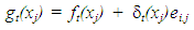
Pakistan is situated in Asia between 23.30 degrees and 36.45 degrees Latitude (N) and 61 degrees and 75.45 degrees Longitude(E). Pakistan is bounded by the three world famous mountainous ranges, which play an important role for summer and winter precipitation. In the northwest lies the Hindukash Range, in north lies the central Karakaram Range and in northeast lies the Himalayan regions of Pakistan. The country has four seasons

i. Summer (May to mid-September)

ii. Autumn (Late September to November)

iii. Winter (December to February)

iv. Spring (March, April)

Climatic Regions of Pakistan

The climate of Pakistan on the whole is dry and extreme; summers are extremely hot and winters are extremely cold with little rainfall during the year. The climate varies from place to place, therefore, Pakistan may be divided into the following four distinct zones:

i. The North and North Western Mountainous Area

This Region consists of the North and the North-Western Mountainous areas. This region has a very severe winter and the temperature falls below freezing point. In this area the winter season extents from six to eight months. On the other hand, summers in this region are very pleasant.

ii. The Upper Indus Plain

Below the Northern Mountainous Area is the upper Indus Plain. In this area the summer is very hot. The months of May, June, and the first week of July are very hot because of absence of rainfall. However, the climate here becomes pleasant when rain falls in July. The winter season is very pleasant but it not last long.

iii. The Coastal Areas and Lower Indus Valley

The temperature in the coastal areas and the lower Indus Valley does not rise due to sea land breeze. In this region rain is scarce; however, during sea breeze conditions, humidity is found in the air. Sea breeze keeps the climate pleasant. There is not much difference in the temperature among the different months.

iv. The Plateau of Baluchistan and the Thar Desert

In summer, the temperature in the Plateau of Baluchistan and the Thar Desert rises and most of the Mountainous regions of Baluchistan are dry and hot. The winter season is very severe in Baluchistan and sometimes snow falls in certain parts. Pakistan is basically an agricultural country as most of its economy depends upon agriculture. The country has developed the world’s largest contagious canal network. Monsoon precipitation is the lifeline of Pakistan which not only caters the national power supply and standing crops water demands but help gathers the reserve to meet the requirement of low flow period in the next 4-5 months. Rainfall plays an important role in agriculture so early prediction of rainfall is necessary for the better economic growth of the country. Prediction of rainfall contributes to crops development and harvesting sufficiency in water supply and water resource policy.

The climate of Pakistan is generally characterized by hot summers and cool or cold winters. Also it has wide variations between temperature extremes at certain locations. As said earlier, Pakistan has four seasons: a cool and dry winter from December through February; a hot and dry spring from March through May; the summer/rainy season from June through September; and the retreating monsoon period of October and November. The duration of these seasons vary somewhat according to location. Generally, there is little rainfall all over the country. Half of the annual rainfall occurs in July and August, while the remainder of the year has significantly less rain.

Figure 1 depicts the map of Pakistan with several regions according to rainfall (Source: http://www.globalcitymap.com/Pakistan). From this map, it is clear that most of the areas have little rain, and heavy rain occurs mostly in the Northern areas. Some parts of the provinces Sindh and Punjab and a huge part of Baluchistan are extremely dry with average rainfall of below 5 inch units (127 mm).

Figure 1. Map of Pakistan with different regions according to rainfall (Source: http://www.globalcitymap.com/pakistan)

In this research, secondary dataset of average rainfall comprising 115 years (1901 to 2015) were acquired from the World Bank website (www. http://sdwebx.worldbank.org). The data are transformed as sliced functional time series (SFTS) then several time series models were applied to forecast the average rainfall in Pakistan. The techniques used are described below:

Sliced Functional Time Series (SFTS) and Outlier Detection

The functional time series (FTS) models were first introduced by Hyndman and Ullah (2007). Initially, the aim was to model the log mortality and fertility rates. Using this method, the functional curves are observed (with error) at time t = 1,…,m, and we wish to forecast the functions for times t = m+1, …m+h. Let [g_t(x_j)] denote the observed data, where j = 1,…p. We assume that there are underlying L₁ continuous and smooth functions [f_t(x)] such that

(1)

where [e_i.j] are independent and identically distributed random variables with zero mean and unit variance, and δ_t(x_j) allows for heteroskedasticity.

The Hyndman and Ullah (2007) technique uses non parametric smoothing on each curve g_t(x) separately to obtain estimates of the smooth functions [f_t(x)]. Panelized regression splines (Wood 1994) are used for smoothing, and then a functional principal component approach (Ramsay and Silverman 2005) is used to decompose the time series of functional data into a number of principal components and their scores. The functional time series (FTS) model can be written as follows:

(2)

where Ψ_k(x) is the k^th principal component, the set of coefficients [α_1,k ,…. α_m,k] are the corresponding scores, e_t(x) denotes the independent and identically distributed random functions with zero mean, and K is the number of principal components to be used.

Hyndman and Shang (2009) proposed three new graphical methods for plotting the functional time series. They include the rainbow plot, the functional bagplot and the functional highest density region (HDR) boxplot. A side benefit of their approach is the identification of outliers, which may not be obvious from the plot of the original data. These outliers are either magnitude outliers (i.e the curves lie outside the range of the vast majority of the data), or they may be the shape outliers (the curves that are within the range of the rest of the data) but they have different shape from other curves. It is also possible that the curves may exhibit a combination of these two features. The presence of the outliers may have serious effect on the modeling and forecasting series.

To detect the outliers from a functional time series, the first step is to obtain the functional curves, then the data are transformed into sliced functional time series (SFTS). For this, the entire data are sliced for each year as a function of 12 months. These curves are plotted in rainbow order with red for the earlier years and violet for the most recent years. The functional curves are then projected into a finite dimensional subspace. The subspace R² is chosen for simplicity. Based on Tukey’s (1974) halfspace bagplot and Hyndman’s (1996) HDR boxplot, each of the functional data point in R² are ordered by data depth and data density. Those curves that have either lowest depth or lowest density are considered to be the outliers (the reader is referred to Hyndman and Shang (2009) for details).

Functional Bagplot

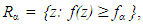
The functional bagplot is based on the bivariate bagplot of Rousseeuw et al. (1999), applied to the first two principal component scores. It uses Tukey's (1974) halfspace location depths. 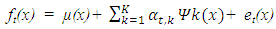The depth region R_k is the set of all , with Since the depth regions form a series of convex hulls, we have for The Tukey bivariate depth median is defined as the value of , which minimizes if there is such a unique , otherwise it is defined as the center of gravity of the deepest region.

Functional HDR boxplot

The functional HDR boxplot is based on the bivarate HDR boxplot (Hyndman, 1996), which is applied to the first two principal component scores. The bivariate HDR boxplot is constructed using a bivariate kernel density estimate f(z), which is defined as

(3)

where Z_i represents a set of bivariate points, K_hi(^.) = K(^./hi)/hi, K is the kernel function, and h_i is the bandwidth for the ith dimension. The bandwidths were selected using smoothed cross validation (Duong and Hazelton, 2005). Using the kernel density estimates, a HDR is defined as

(4)

where f_α is such that ∫_Rαf(z)dz=1-α; that is, it is the region with probability of coverage 1- α, where all points within the region have a higher density estimate than any of the points outside the region, hence the name “highest density region”.

3. Results and Discussion

Figures 2 and 3 represent the daily and the monthly plots of the series which show a clear seasonal pattern. The precipitations are higher for July and August but relatively less for the other months. It can also be observed that the amount of rainfall is continuously decreasing in the recent years, especially after 1980. In order to see a clearer picture of the series, this is divided into the groups of 30 years, as shown in Figure 4.

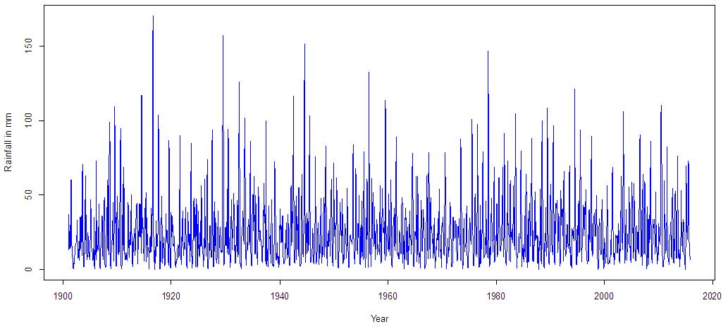Figure 2. Plot of monthly rainfall in different areas of Pakistan during 1901-2015

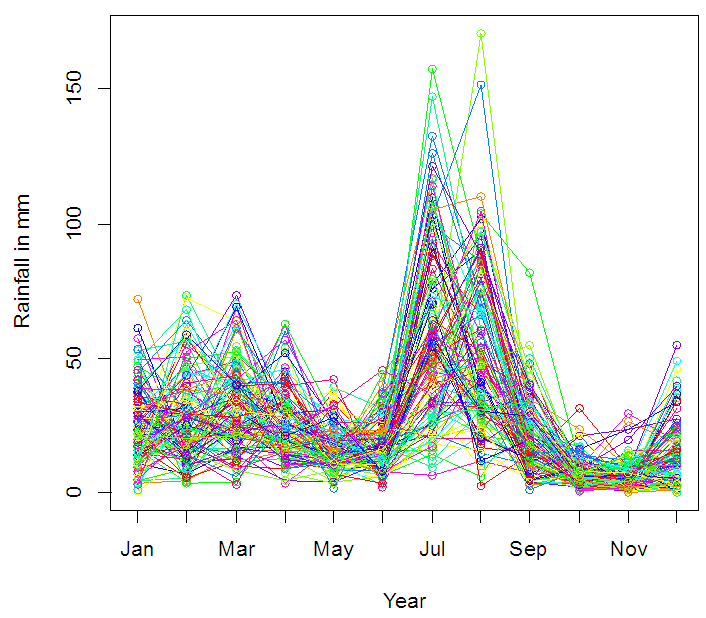Figure 3. Plot of monthly rainfall in Pakistan during 1901-2015. These are 115 curves, each representing a single year

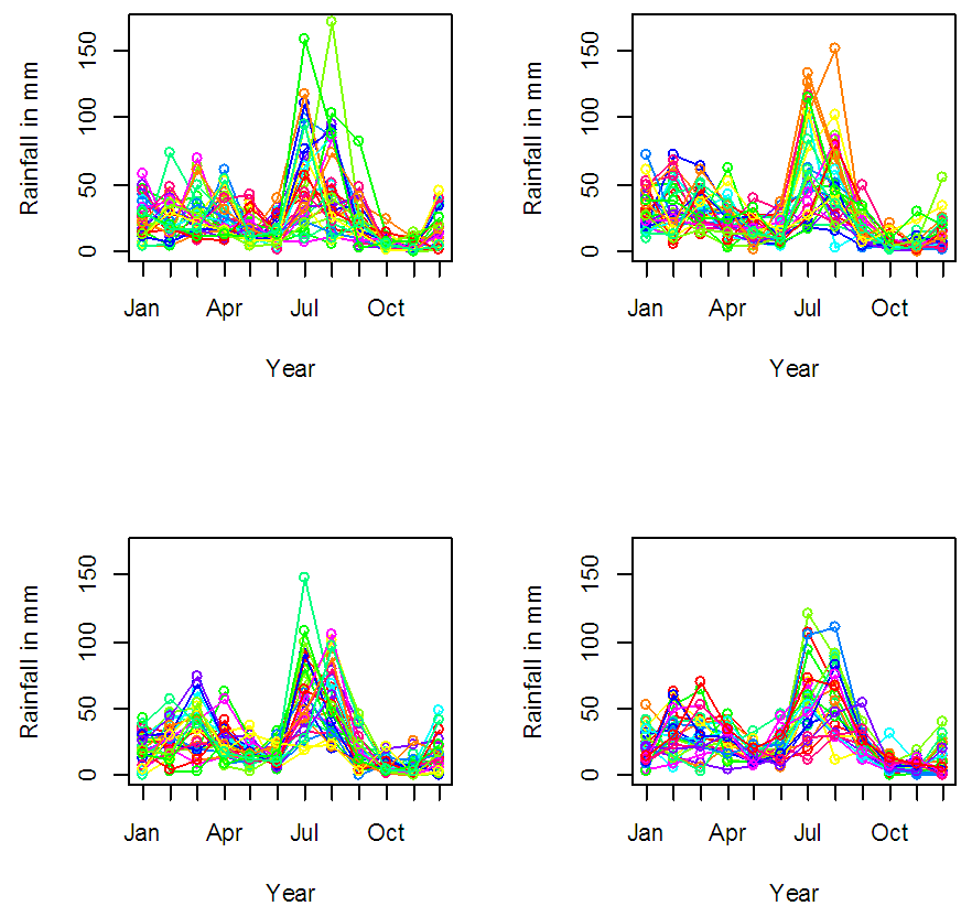Figure 4. Season plots for rainfall during (1901-1930), (1931-1960), (1961-1990) and (1991-2015)

It is clear that the amount of rainfall was higher during 1901-1960, even for the months of Jan-March but not that high amounts in these months since last 50 years. In order to select a better forecasting time series model, we consider the data from 1951 to 2015. After the independence of Pakistan in 1947, most of the jungles were cut down; hence this may one of the reasons to the decline in rainfall.

Figure 5 depicts the amount of rainfall during (1951-2015). The months of July and August have heavy rain due to the monsoon whereas the other months are having relatively low precipitations. There is little rain in the months of May, June, October and November in northern areas with about no rain in Sind and Baluchistan in these four months. Hence the amount of average rainfall is lower in these four months while October is considered to be the driest month in Pakistan.

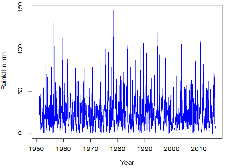Figure 5. As in Fig. 2, but during 1951-2015

Next, the data are transformed into sliced functional time series. The first step is to obtain the functional curves. For this, the entire data are sliced for each year as a function of 12 months, as plotted in Figure 6. These curves are plotted in rainbow order with red for the earlier years and violet for the most recent year. We use R statistical software, with R package rainbow (Hyndman and Shang 2009) for this plot.

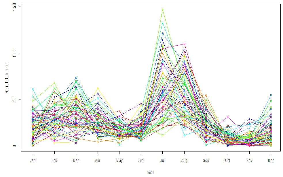Figure 6. Plot of average rainfall during (1951-2015) as Sliced Functional Time Series. The curves for each of the 65 years are plotted in the colors of a rainbow, as function of the month

The functional curves are then projected into a finite dimensional subspace. The subspace R² is chosen for simplicity. Based on Tukey’s (1974) halfspace bagplot and Hyndman’s (1996) HDR boxplot, each of the functional data point in R² is characterized by data depth and data density. Those curves that have either lowest depth or lowest density are considered to be the outliers (the reader is referred to Hyndman and Shang (2009) for details).

Figures 7 and 8 represent the functional bagplot and functional HDR plot, whereas figure 9 depicts the functional bivariate plot. These plots showed that 1956, 1978 and 2010 are the outliers. Different components of FTS models and sliced functional time series forecasts are plotted in Figure 10 and 11 respectively. Figures 12 and 13 show the forecasts obtained from ARIMA and Exponential smoothing stat-space models.

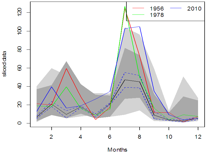Figure 7. Functional bagplot for rainfall data. Median curve is denoted by black color, along with its confidence interval (blue dotted lines). The outliers are represented by red, green and blue colors. Inner and outer regions are plotted in dark grey and light grey color respectively

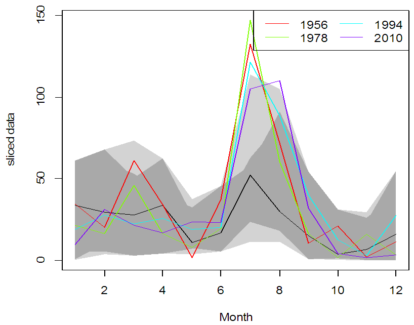Figure 8. Functional HDR plot for rainfall data. Black represents the modal curve, whereas the outliers are represented by red, green and blue colors. Inner and outer regions are plotted by dark grey and light grey color, respectively

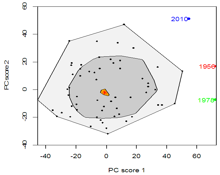Figure 9. Functional bivariate plot for rainfall data with first two principal components being plotted. The Red asterisk is the sample median, whereas the inner and outer regions are plotted by dark grey and light grey color, respectively

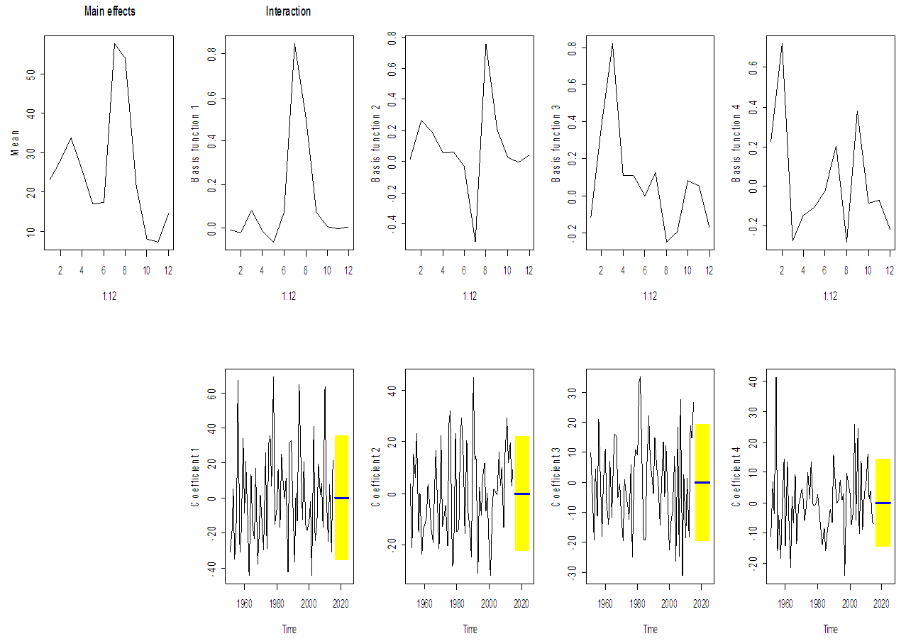Figure 10. Different components of FTS models applied to the rainfall data, along with 10-year forecasts and 80% prediction intervals of the time series coefficients

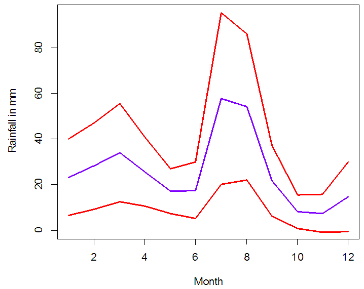Figure 11. Sliced Functional Time Series Forecasts of monthly average rainfall in Pakistan (blue color), along with 80% prediction intervals (red color)

Figure 12. 10-year forecasts (2016-2025) of average rainfall in Pakistan using ARIMA model, along with 80% prediction intervals

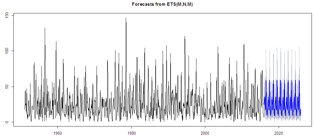Figure 13. As in Fig. 12, but using Exponential Smoothing State Space model

Finally the forecasting performance of the models will be measured by Mean Error, Root Mean Square Error (RMSE), Mean Absolute Error (MAE), Mean Percentage Error (MPE) and Mean Absolute Percentage Error (MAPE). These measures are defined as follows:

1. Mean Error (ME) = mean(|e_i|) where e_i is the forecast error;

2. Root Mean Square Error (RMSE) =

3. Mean Absolute Error (MAE) = mean(|e_i|)

4. Mean Percentage Error (MPE) = mean(p_i) where pi =100e_i/y_i

5. Mean Absolute Percentage Error (MAPE) = mean(|pi|)

The rainfall data from January 1951 to December 2015 is divided into two subsets: a training set January 1951 – December 1995 and test set January 1996– December 2015. The training subset is used to fit the three models ARIMA, ETS and SFTS, and to estimate the parameters. The second subset is used for comparing the forecasts from different models. The results are shown in Table 1. Table 2 gives the average rainfall forecasts from 2016-2020 along with 80% prediction intervals.

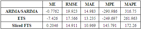Table 1. Out of sample forecasting performance of different models using mean error (ME), root mean square error (RMSE), mean absolute error (MAE), mean percentage error (MPE) and mean absolute percentage error (MAPE)

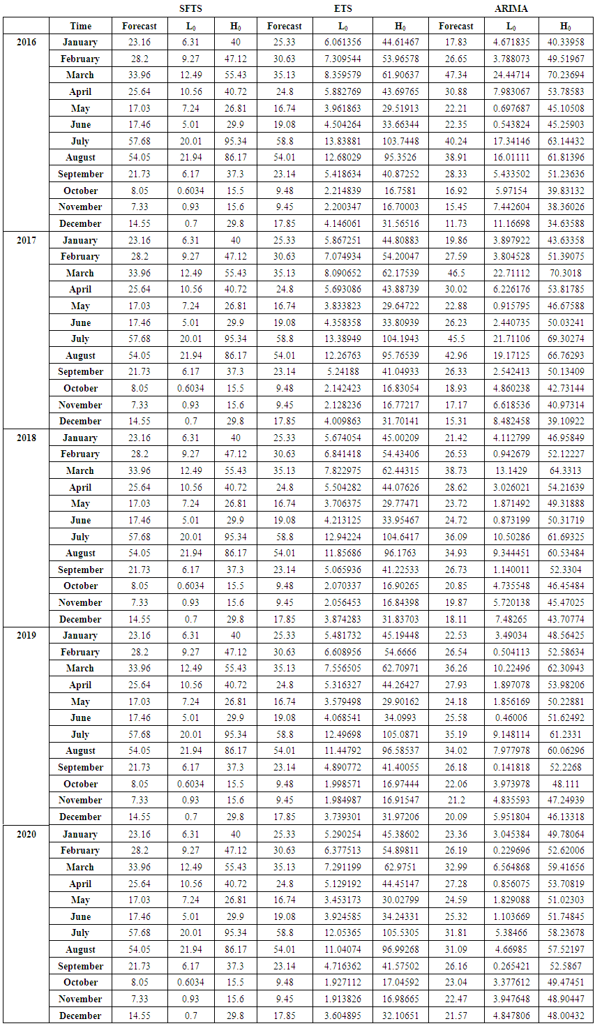Table 2. Average rainfall forecasts obtained from Sliced Functional Time Series (SFTS), Exponential Smoothing State Space (ETS) and ARIMA models along with 80% prediction intervals. L0 and H0 are the lower and upper prediction limits

4. Discussion

In Pakistan, adverse consequences of rainfall have already been observed. They are in the form of droughts and super floods which have badly affected human settlements, water management and agriculture. The majority of Pakistan’s 180 million people live along the Indus River that is prone to severe flooding in July and August. Major earthquakes are also frequent in the mountainous northern and western regions. Measures to improve cultivation outputs and resilience to climate variation have long been underway, but a substantial push is still needed as amply demonstrated by the 2010 devastating floods. Priority areas for research and adaptation measures include the water, infrastructure, energy, and agriculture sectors, with particular attention to reducing vulnerability to flooding and improving water management in the Indus Basin.

In this paper, monthly rainfall data were analyzed through the sliced functional time series (SFTS) model, a relatively new method of forecasting was introduced and the monthly forecasts for the next ten years (2016-2025) were obtained along with 80% prediction intervals. These forecasts were also compared with the forecasts obtained from Autoregressive Integrated Moving Average (ARIMA) and exponential smoothing state space (ETS) models. It was found that the SFTS model performed better than standard ARIMA and ETS ones and the forecasts obtained from SFTS models are not only more accurate and reliable, but they also provide narrow prediction intervals as compared to other models.

ACKNOWLEDGEMENTS

The authors are thankful to the two anonymous referees for their valuable suggestions which improved the work considerably.