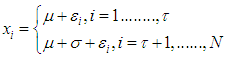
-
Paper Information
- Paper Submission
-
Journal Information
- About This Journal
- Editorial Board
- Current Issue
- Archive
- Author Guidelines
- Contact Us
World Environment
p-ISSN: 2163-1573 e-ISSN: 2163-1581
2017; 7(1): 10-22
doi:10.5923/j.env.20170701.02

Khronostat Model as Statistical Analysis Tools in Low Casamance River Basin, Senegal
 Abstract
 Reference
 Full-Text PDF
 Full-text HTML
Vieux Boukhaly Traore1, Mamadou Lamine Ndiaye2, Cheikh Mbow3, Giovani Malomar4, Joseph Sarr3, Aboubaker Chedikh Beye1, 4, Amadou Tahirou Diaw2
1Hydraulics Laboratory and Fluid Mechanics, Cheikh Anta Diop University, Dakar, Senegal
2Geoinformation Laboratory, Polytechnic High School, Cheikh Anta Diop University, Dakar, Senegal
3Fluid Mechanics and Applications Laboratory, Cheikh Anta Diop University, Dakar, Senegal
4Physics Solid and Sciences of Materials Laborator, Cheikh Anta Diop University, Dakar, Senegal
Correspondence to: Vieux Boukhaly Traore, Hydraulics Laboratory and Fluid Mechanics, Cheikh Anta Diop University, Dakar, Senegal.
| Email: |  |
Copyright © 2017 Scientific & Academic Publishing. All Rights Reserved.
This work is licensed under the Creative Commons Attribution International License (CC BY).
http://creativecommons.org/licenses/by/4.0/

Spatial monitoring of climate behavior through rainfall variability is important step for the better understanding of the water resources in the river system. This paper aims to highlight rainfall variability at yearly scale and identify the various climate situations and characteristics of the study area during studied chronicle in the lower valley of the Casamance river basin. Three rainfall stations Ziguinchor, Bignona and Oussouye over the period of 55 years on average acquiring from ANACIM database (National Agency of Civil Aviation and Meteorology), have been selected for this purpose. Choice of rainfall is due to the fact that it is a key variable in West Africa in general and more specifically over the Sahel region where economies, livelihoods and food security are highly dependent on rained agriculture. To reach our objective, we have proceded through some analysis based on rupture detection testing (Pettitt, Hubert, Buishand and Lee and Heghinian test) and randomness testing (Autocorrelogram and correlation test of Rank) at the 5% significance level, while using the Khronostat software. Results show decreasing shift and randomness for all three stations the probabilities of this break are given by Lee and Heghinian test and are equal to 0.57142 for Ziguinchor, 0.354188 Bignona and 0.2846 for Oussouye. Rupture detection test indicate the same shift date established in 1967 for all stations. This study provides interesting opportunities to climate experts and water stakeholders in understanding the link between climate instability and water availability, thus contributing to the sustainable management of water resources.
Keywords: Climatic events, Rainfed agriculture, Statistical approach, Climate monitoring, Sustainable water resources, Food safety
Cite this paper: Vieux Boukhaly Traore, Mamadou Lamine Ndiaye, Cheikh Mbow, Giovani Malomar, Joseph Sarr, Aboubaker Chedikh Beye, Amadou Tahirou Diaw, Khronostat Model as Statistical Analysis Tools in Low Casamance River Basin, Senegal, World Environment, Vol. 7 No. 1, 2017, pp. 10-22. doi: 10.5923/j.env.20170701.02.
Article Outline
1. Introduction
- Nowadays, sustained interest manifests itself around the climate change and its increased variability, because of sometimes tragic consequences they can cause on ecosystems, environment and populations (Beyene and al., 2013). According to (Biazen, 2014), the severity of climate variability and change profoundly influence social and natural environments throughout the world. He indicates also that climate change strongly influences forest productivity, species composition, and the frequency and magnitude of disturbances that impact forests. This is why (Piyoosh and Bhavna, 2015) affirms that climate change is one of the most serious threats that humanity may ever face. According to (Barbé et al., 2002), climatic events (change and variability) concern mainly a blend of several factors that are naturals and/or anthropic orders. (Emmanuel, 2013) defined basically climate as the average weather conditions of a particular neighborhood observed over a period of together. The climatic water cycle is one of the major manifestations of the climate; therefore, its monitoring will allow apprehending certain aspects of climate evolution. (Ouarda and al., 1999) indicate that the adapted variables to the climate monitoring are: river flows, lake levels, rainfall, temperatures, the groundwater level According to (Doumouya and al., 2016; Ndiaye and al., 2016), among these variables, rainfall represents the most important climate factor for population, environment and ecosystems. (Halmstad and al., 2012; Yao and al., 2012) reveal that rainfall plays a key role in the planning and management of sustainable water resources, particularly as the fundamental design parameter for dam safety and flood risk analyses) and (Hadgu and al., 2013) add that rainfall is the main source of water for crop production as irrigation covers only 5% of the cultivated land in many African countries. Most of the water resources projects are designed based on the historical pattern of water availability and demand, assuming constantly climatic behavior (Abdul and al., 2006). So, any change in the climate behavior has a big influence in the precipitation regimen (Maftei and al., 2010). According to (Kingumbi and al., 2005; Masoud and al., 2016), the existence of an increasing or decreasing trend in hydrological time series can also be explained by the changes of the factors that influence the precipitation. Many work at worldwide scale, have highlighted the negative effect of climate fluctuations on rainfall and flow (Kouassi and al., 2008 and 2010). They are mainly characterized by a decrease of the quantity, frequency of rainfall in time and space and a change in timing of occurrence (Kharin and Zwiers, 2000; Huntingford and al., 2003), seasonal changes of rainfall, changes of basin response, causing a rise of temperature (Kingumbi et al., 2005). Many investigations have revealed that variability and change of climate are major threats for developing countries (Sambou and al., 2009). According to (Biazen, 2014), poor households are not only located in high-risk areas, but suffer lack of economic and social resources According to (Elbouqdaoui and al., 2006; Rosine and al., 2014) Sahelian countries are the most affected, due to the impact on rainfed agriculture. This is explained by a low level of economic and social development, education, training for farmers, weakness of agricultural equipment, fragile ecosystems and especially the dependence of people to natural resources (Hadgu and al., 2013). Climate implications on those water resources in West Africa are particularly strong (Payne and al., 2004; Christensen et al., 2004), and affect, in turn, numerous activities sectors industries both economic development (agriculture, industry, hydropower) and for the future of the populations (health, drinking water supply, food security) (Servat and al., 1999; Fulvie and al., 2009; Traore et al., 2015). (Goulden and al., 2009) reported that the impact of future climate change on hydrographic freshwater systems will It will amplify problems caused by other constraints such as population growth, changing economic activity, changes in land use and level of urbanization and adding, water demand (irrigation, household consumption, hydropower) will increase in the coming decades. According to (Radinovié and Curié, 2009), future climate change would influence all characteristics of rainfall in terms of intensity, frequency and duration. So, to try to elucidate this problem of water lack, it is essential to analyze the rainfall series and evaluate the effect of their gradual reduction (or not), taking into account climatic conditions. It is for these reasons that climate and increased climate variability have recently become a pressing issue in various development, environment, and political forums at the national, regional, and international levels (Hua Chen and al., 2007). It is through these meetings, to understand the dynamics of climate and to think in terms of reliable assessments of the impact of climate hazards on natural resources in order to develop adaptation strategies and appropriate forecast to the new environmental conditions (Beyene and al., 2009; Maurer and al., 2009; Conway and al., 2011). Many works in West Africa, have identified and characterized the magnitude of climate fluctuations from the rainfall series (Servat and al., 1997). These researches are generally are related to statistical tests based on the detection of breaks, trends and their directions. (Lubès and al., 1998). A comprehensive analysis of these characteristics can improve an understanding of variations and changes in rainfall and therefore in the climate patterns (Khon and al., 2007). However to ensure the quality of the results and conclusions on the study of climate change increased climate variability and its impacts, the check for quality and reliability of data, is a priority and mandatory (Traore and al., 2014). Nowadays, there are several methods and tools using the hydro climatic series for statistical studies (Feuillet, 2009; Hubert, 2000). These require methodological rigor and should lead to conservative interpretation (Machiwal and Jha, 2008). Therefore the choice must be made by identifying tools and/or methods able to accurately highlight all the events related to climate variability and change and their impact on water resources to ensure prediction (Vezzoli and al., 2012). In this paper, we limited on the watershed of Low Casamance, southern Senegal. The choice of this valley is linked to the fact that more than 90% of the people of this locality live from rain-fed agriculture. In that respect, we have proceded through some analysis based on statistical tests of independence (autocorrelogram test, correlation test of Rank) and homogeneity (Pettit, Hubert, Lee and Heghinian and Buishand ellipse tests) applied to an annual chronological rainfall series of Ziguinchor, Bignona and Oussouye raingauges. These data were acquired from the database of ANACIM (National Agency of Civil Aviation and Meteorology) that guarantees its quality and reliability. The Khronostat software which allows such analysis, was used to characterize the series (random or not), detect abrupt changes of the characteristics in distribution law of the series and identify the direction and magnitude of the tendency. Statically speaking, climate change assumes long-term degradation of the average values of the statistical characteristics of studied variables over long periods of time while climate variability assumes stationary and describes the fluctuation of the seasonal or annual values compared to the reference time values (Ouarda and al., 1999; Servat and al., 1997). Whatever, the possible evolutions of these climate variables can be reduced to two types of changes to be analyzed: the change in the average and the variance (Lubès and al., 1998). The purpose through these statistical methods is to bring specific elements of knowledge about events in terms of variability and climate instability and its relationship to that of water resources. Our motivation at this level is to bring specific elements of knowledge about events in terms of variability and climate instability and its relationship to that of water resources. This would from development of different climate scenarios to help estimate and sustainable water resources management.
2. Materials and Methods
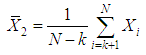
2.1. Study Area
- Casamance is a natural area of Senegal in south-west between latitude 12° 20' 13° North and longitude 16° 16° 50 'West with a total area of 52 000 km2 on 200km length (Fig.1). It is limited to the north by Gambia to the south by Guinea Bissau and Guinea, east by Mali and to the west by the Atlantic Ocean. It is partially isolated from the rest of the country by the Gambian territory (Cormier, 1991). Casamance is composed of Low Casamance, middle Casamance and high Casamance. Low Casamance on which focuses this study, covers an area of 7300 km2 and encompasses the departments of Ziguinchor (1153 km2), Oussouye (891 km2) and Bignona (5295 km2) (Diatta, 2001). The climate is tropical subguineen type with a strong maritime influence and two seasons: a dry season from November to May and a rainy season from June to October. August is the rainiest month (Olivry, 1987). Average annual rainfall is about 1200mm at Ziguinchor raingauge, 1300mm at Bignona raingauge and 1600 at Oussouye raingauge (Dacosta, 1992). Minimum temperatures range from 12°C to 20°C from December to February. From October to November and March to April, the maximum temperatures turn around 26°C. From July to September, they can reach 33°C. The average temperature is estimated at 27°C. From November to April, the prevailing winds are from North to Northwest sector although we note the presence of hot dry winds. The monsoon moved from May to October. This southwestern wind sector is the main vector of rain (Sagna and Touré, 1997). Evaporation plays an important role in the current evolution of ecosystems of Casamance, because it is largely responsible for the increased salinity of the river during periods of rainfall deficit by concentration of seawater. The maximum is located in February (about 150 mm) and the minimum in July (about 50 mm) (Lamagat and Loyer, 1986).
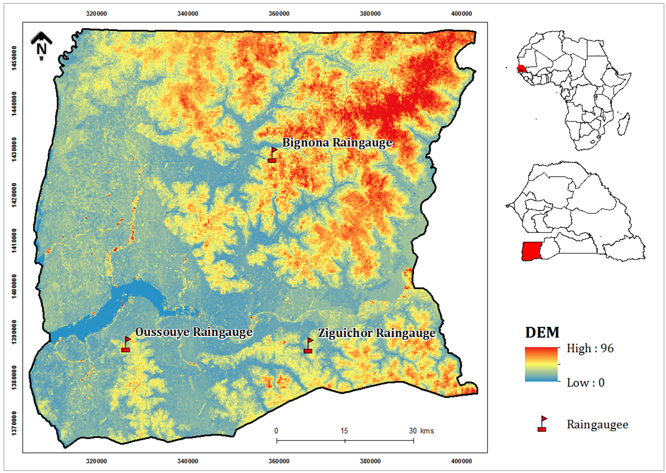 | Figure 1. Localisation of low Casamance river basin |
2.2. Philosophy and Principle of a Statistical Test
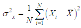
- A statistical test is to make a decision based on information collected on a sample (Lemaitre, 2002). The tests are to determine if a characteristic (average or standard deviation) taken from a sample, is identical to a reference (standard) or that of another sample. A statistical series can be characterized by two types of parameters: i) position parameters (median, average, ...): they give the order of magnitude of the observations and are related to the central tendency of the distribution and ii) dispersion parameters (standard deviation, variance, coefficient of variation): they show how observations fluctuate around the central tendency (Mestre, 2000). Ordinarily, tests are ranged in two categories: i) the parametric tests that test the value of a certain parameter, in this case, the characteristics of the data can be summarized using the estimated parameters of the sample, subsequent testing procedure bears then on these parameters and ii) nonparametric tests that do not involve parameters and make no hypothesis on the distribution of variables; the prior step is to estimate the parameters of the distributions before proceed to hypothesis test itself. Whatever the test category used, the goal is to decide between two hypotheses, one called null or fundamental (denoted by H0) and other called alternative (denoted by H1). A hypothesis is an attempt to explain how a phenomenon works or approach consisting of the assessment based on a data set (sample). In general, the null hypothesis corresponds to a stationary situation while the alternative hypothesis reflects a change (break or trend) (Lubes and al., 1998). The fundamental notion on testing, the probability that one has to be wrong. There are two ways to go wrong in a statistical test: i) wrongly reject the null hypothesis H0 when it is true: it is the first type of risk (or Type I error) and in general there is the probability α of being wrong in this direction and ii) accept the null hypothesis when it is false: it is the risk of the second kind (or type II error) and in general there is the probability of β err in that direction. The ideal solution is to minimize these types of errors, but in a sample, if we reduce the a, increases the other (Lubes et al., 1994). In practice we minimize the error type I, this type of error is assigned a probability α. This is the probability of making the Type I error is called the level of significance of the test; it helps to define the test of confidence. Knowing this probability α, we can deduce that for the error of β type II which is of the form (1 - α) (Bobée, 1978). The different stages of a statistical test are: i) to define the null H0 (hypothesis testing) and the alternative hypothesis; ii) calculating the value of the decision variable from the data; iii) define the level of significance of the test (denoted α); iv) read on the table the reference value of the variable depending on the test used and v) take a decision regarding the assumption made and make an interpretation: it is to reject or accept the null hypothesis H0. (Fig.2) shows the summary diagram.
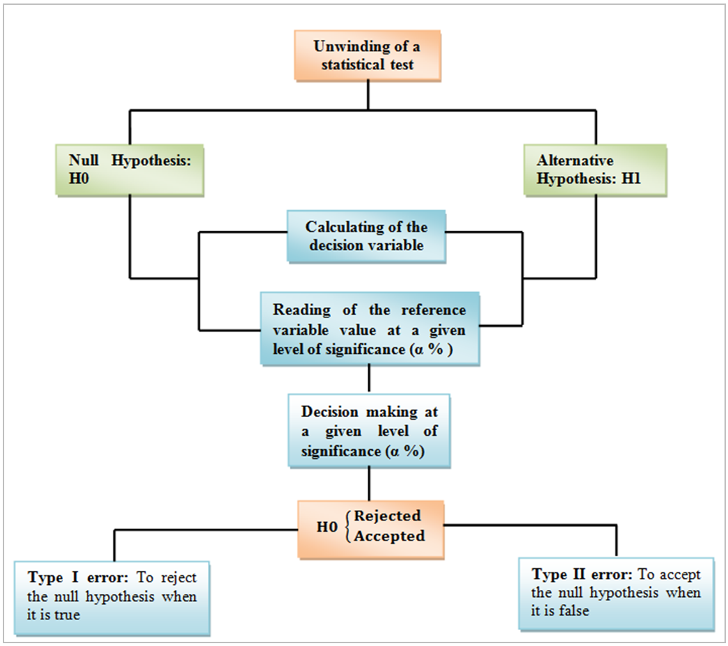 | Figure 2. Organization of statistical tests |
2.3. Description of Khronostat Model
- Khronostat is a statistical model developed by IRD (Research Institute for Development) at the House of Water Sciences (MSE) of Montpellier. It was developed as part of a study on climate variability in West and Central Africa and is oriented on the analysis of hydroclimatic series (Boyer, 2002). It can evolve on an annual, monthly or daily scale depending on the needs expressed. Khronostat includes within it various statistical tests: i) the first test category concerns the randomness (or independence test) series (correlation test on the rank and autocorrelogram test): they carry to the constancy of the average of the series throughout its observation period and ii) the second test category concerns the homogeneous character of the series (Pettitt test, Buishand test, Hubert test, Bayesian methods or Lee & Heghinian test): they relate to the detection of breaks in a time series (Paturel, 1995). These tests, whose application conditions are not very strict: i) allow to characterize as well as possible the evolution of climate parameters; (ii) identify the pivotal years of climate change; (iii) complement climatic index calculations and iv) define the causes of series heterogeneity by sudden changes in climate series. Khronostat is adapted to all variables (climatic, hydrological, meteorological,..). However, it requires complete series with no gaps. Its choice in this study is justified by the robustness of its tests and also by its success through several similar studies in sub-Saharan Africa. It is also well advised by the meteorologists and climatologists over the world for surveillance or monitoring of drought.
2.3.1. Independence Test
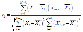
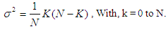
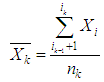
- The independence test is used to test the likelihood of no bond in a population from a sample. It provides information on the strength of the evidence and not on the strength of the association. The most common tests relate to the constancy of the average of the series throughout its period of observation (L’hote and al., 2002). These tests are powerful enough in general to distinguish between random and non-random nature of the series. The independent tests used in this article available in Khronostat are: the correlation test of rank and test the autocorrelogram. For all these tests, the null hypothesis that must be tested is H0 «the series is random» (Bop, 2008). 2.3.1.1. Autocorrelogram TestThe estimation of the autocorrelogram is the first step in the statistical analysis of time series. The autocorrelation coefficient of order k is given by the following expression: The autocorrelation coefficient of the Kth order is given by the equation (1) (Lubès et al., 1994):
 | (1) |
 and
and  are determined for each value of k by equations (2) and (3).
 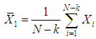 | (2) |
 | (3) |
 | (4) |
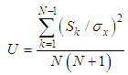
 . The standard score U is given by equation (5) (IRD-Orstom, 1998):
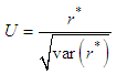 | (5) |
 | (6) |
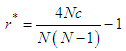
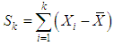
 as
as with (i = 1, j = 2,N), (i = 2, j = 3,N), …, (i = N – 1, j = N).The variance
  is given by the relation (7) (Boyer, 2002):
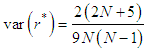 | (7) |
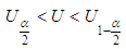 In the case of a tail test, the null hypothesis is accepted when:
  with
with  for a sample size (N> 30). When the series is not random, it can admit a tendency or a periodicity.
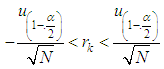
2.3.2. Homogeneity Test
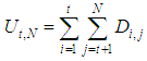
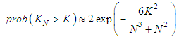
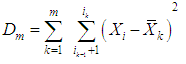
- A sample is said to be homogeneous if it present no breaks. A break can be generally defined as an abrupt change in the probability law of the series at a given time, usually unknown. It corresponds to a trend reversal of the time series (Traore and al., 2014). The break detection tests used in this article and available in Khronostat, are: Pettitt test, Buishand test, Hubert test and Lee and Heghinian test. For all these tests, the null hypothesis that must be tested is H0 « no break in the series » (Paturel, 1995).2.3.2.1. Pettitt Test The Pettitt approach is non-parametric and is derived from the Mann-Whitney test. The absence of break in the series (xi) of size N is the null hypothesis. The use of the test supposes that for any time t with a value between 1 and N, the two time series (Xi) for i = 1 to t and for i = t + 1 to N belong to the same population. The variable that is to be tested is KN, the maximum in absolute terms of the variable Ut,N defined by the relation (8) (L’hote and al., 2002) :
 | (8) |
 | (9) |
 | (10) |
 | (11) |
 | (12) |
 | (13) |
 | (14) |
 | (15) |
 | (16) |
 | (17) |
 are independent and normally distributed, with a mean equal to zero and a variance equal to
  and
and  represent the position in time and the scope of the possible change in the mean respectively. The method determines the a posteriori probability distribution function of the parameters μ and δ, considering their a priori distributions and supposing that the break time follows a uniform distribution. When the distribution is unimodal, the date of the break is estimated by the mode with all the more accuracy as the dispersion of the distribution is small (Boyer, 2002).
3. Application
- In this study, we focus on rainfall because: i) it constitute according to many authors, the most important factor of climate and the most used climatic parameter in reliable diagnosis and analyzes of the climate and its spatial evolution; ii) it plays a key role in the planning and management of sustainable water resources, particularly as the fundamental design parameter for dam safety and flood risk analyses) and iii) it is the main source of water for crop production as irrigation covers only 5% of the cultivated land and the most of the water resources projects in many African countries and especially in Senegal, notably in Low Casamance where agriculture depends entirely on rain; iv) and its time series is complete and without gaps as required by the Khronostat model. Indeed, three rainfall stations, Ziguinchor, Bignona and Oussouye in the lower valley of the Casamance river basin are used over the period 1951-2012, 1950-2012 and 1950-2008 respectively. These were acquired from the database of ANACIM (National Agency of Civil Aviation and Meteorology) that guarantees its quality and reliability. To analyze rainfall variability, we used statistical tests of homogeneity and independence by using Khronostat software. The objective targeted here is, on the one hand, to identify the various climate situations and characteristics of the study area during these chronicles and, on the other hand, to highlight the general rainfall distribution (trends, variability, extremes, etc.) to assess their spatial and temporal extent; such information stand as the basic elements for a deeper reflextion on the phenomena that contribute to the fight against climate change and the knowledge of the link between the instability of the climate and that of water resources; this is an important step for the estimation and sustainable management of water resources.
4. Results and Discussion
- These various tests are performed on three levels of significance or confidence intervals. For this article, the confidence level used is 95%.
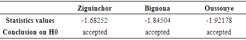
4.1. Results of the Independence Tests
- We present in the Table 1 the results of the rank correlation test and (Fig.3) the result related to autocorrelogram test on rainfall series of Ziguinchor raingauge (Fig.3a), Bignona raingauge (Fig.3b), and Oussouye raingauge (Fig.3ac). It is been observed in the table that all statistics calculated values (in absolute value) is below the reference value 1.96; we conclude then, that the data are stationary, and therefore the null hypothesis H0 «random series», is accepted for these 3 stations. The analysis of Fig. shows that of the 16 calculated values of autocorrelation coefficients, there are 15 for Ziguinchor station; 11 for Bignona station and 10 for Oussouye station which are within the chosen confidence interval. Therefore the null hypothesis «random series», is accepted for these three stations. These results further confirm the results over the previous test related to rank correlation test. We also noticed that the High and low autocorrelation coefficients are respectively located on the 9th and 16th year for Ziguinchor, 2nd and 14th year for Bignona and 2nd and 7th year for Oussouye. H0: null hypothesis «random series»
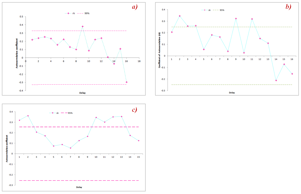 | Figure 3. Autocorrelogram diagram: a) at Ziguinchor raingauge, b) at Bignona raingauge, c) at Oussouye raingauge |
|
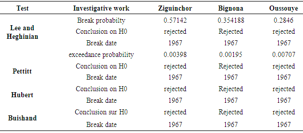
4.2. Results of the Homogeneity Tests
- We present in Table 2 the tabular results of the break detection tests (Lee and Heghinian, Pettitt, Hubert and Buishand) and in Fig.4, 5, 6 and 7 the corresponding graphical results for each station. Analysis of the Table 2 shows that all tests reject the null hypothesis «no break in time series »for each of 4 stations at 5% significance level. According to Lee and Heghinian test, the probability to have a break is equal to 0.57142 for Ziguinchor, 0.354188 for Bignona and Oussouye for 0.2846. The analysis of the graphs shows that all 4 homogeneity tests indicated the same break date corresponding to 1967. Definitively, the rainfall series used are not homogeneous and breakage is more pronounced for Ziguinchor than for Bignona and Oussouye.
|
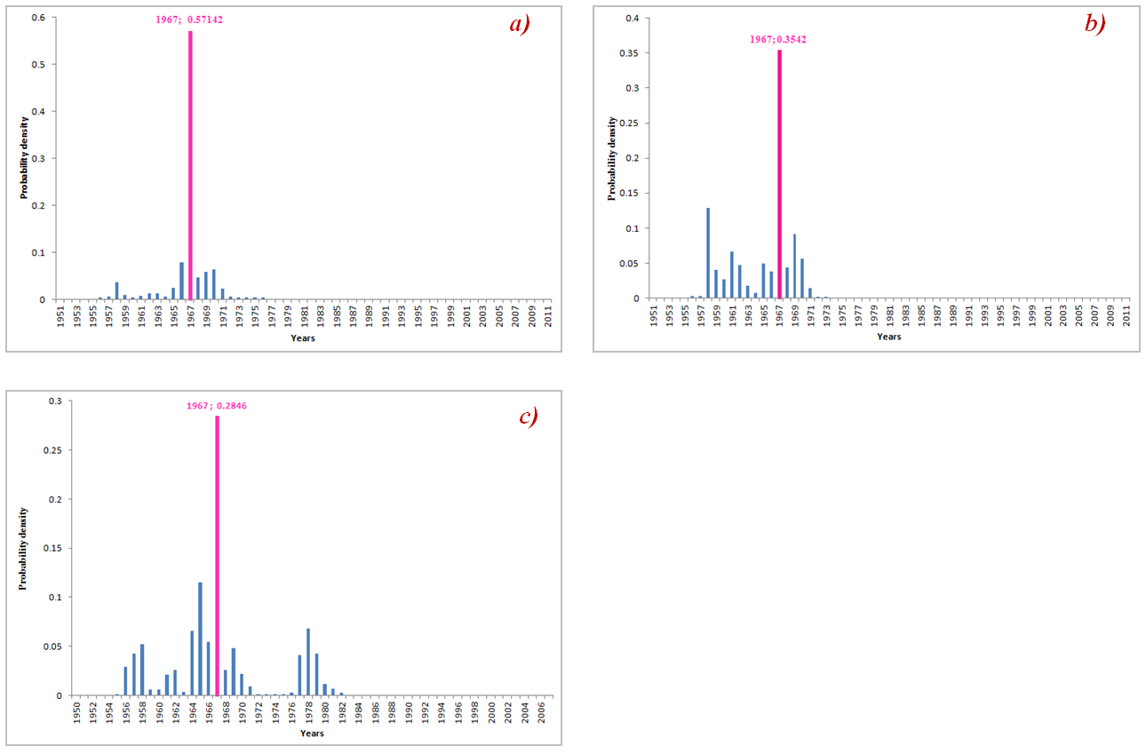 | Figure 4. Lee and Heghinian test diagram: a) at Ziguinchor raingauge, b) at Bignona raingauge, c) at Oussouye raingauge |
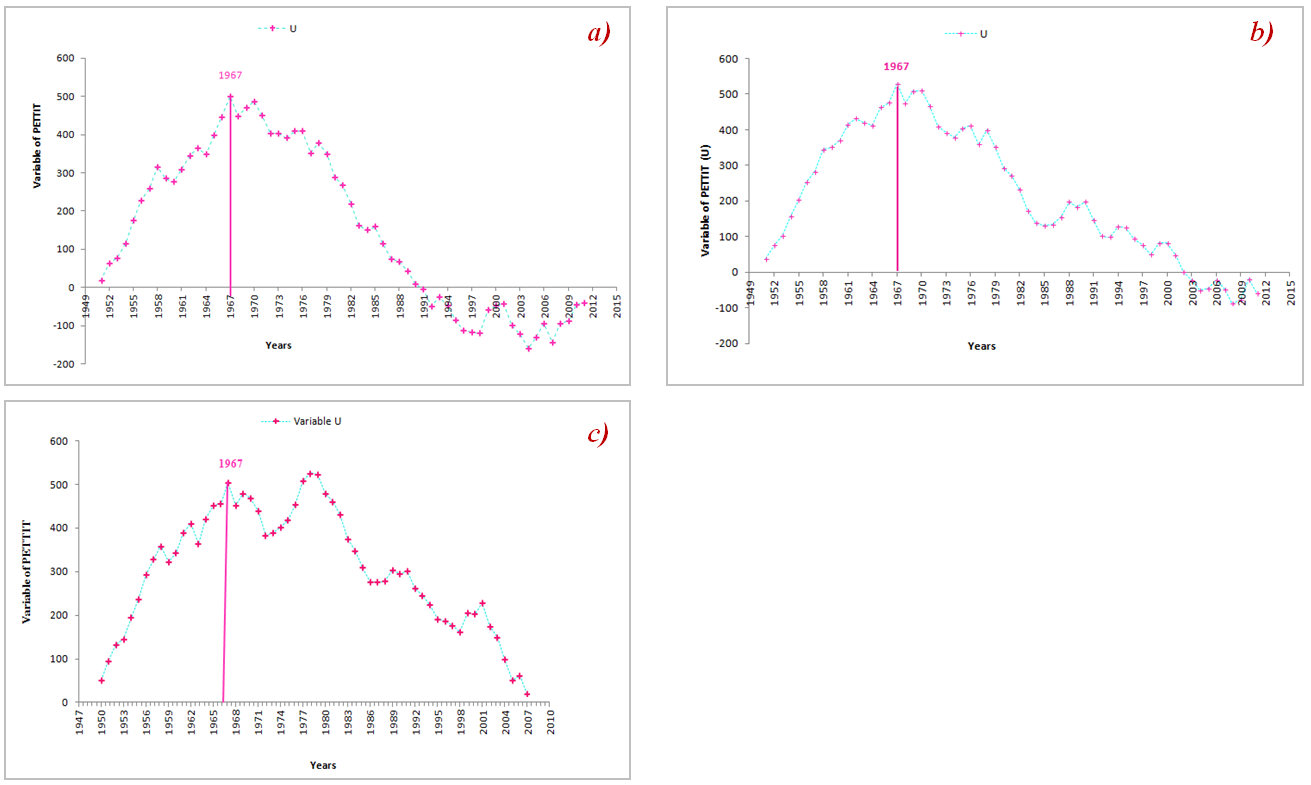 | Figure 5. Pettitt test diagram: a) at Ziguinchor raingauge, b) at Bignona raingauge, c) at Oussouye raingauge |
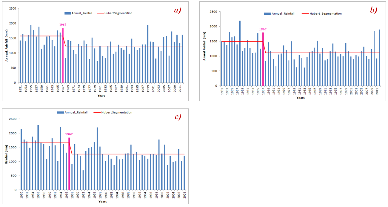 | Figure 6. Hubert segmentation diagram: a) at Ziguinchor raingauge, b) at Bignona raingauge, c) at Oussouye raingauge |
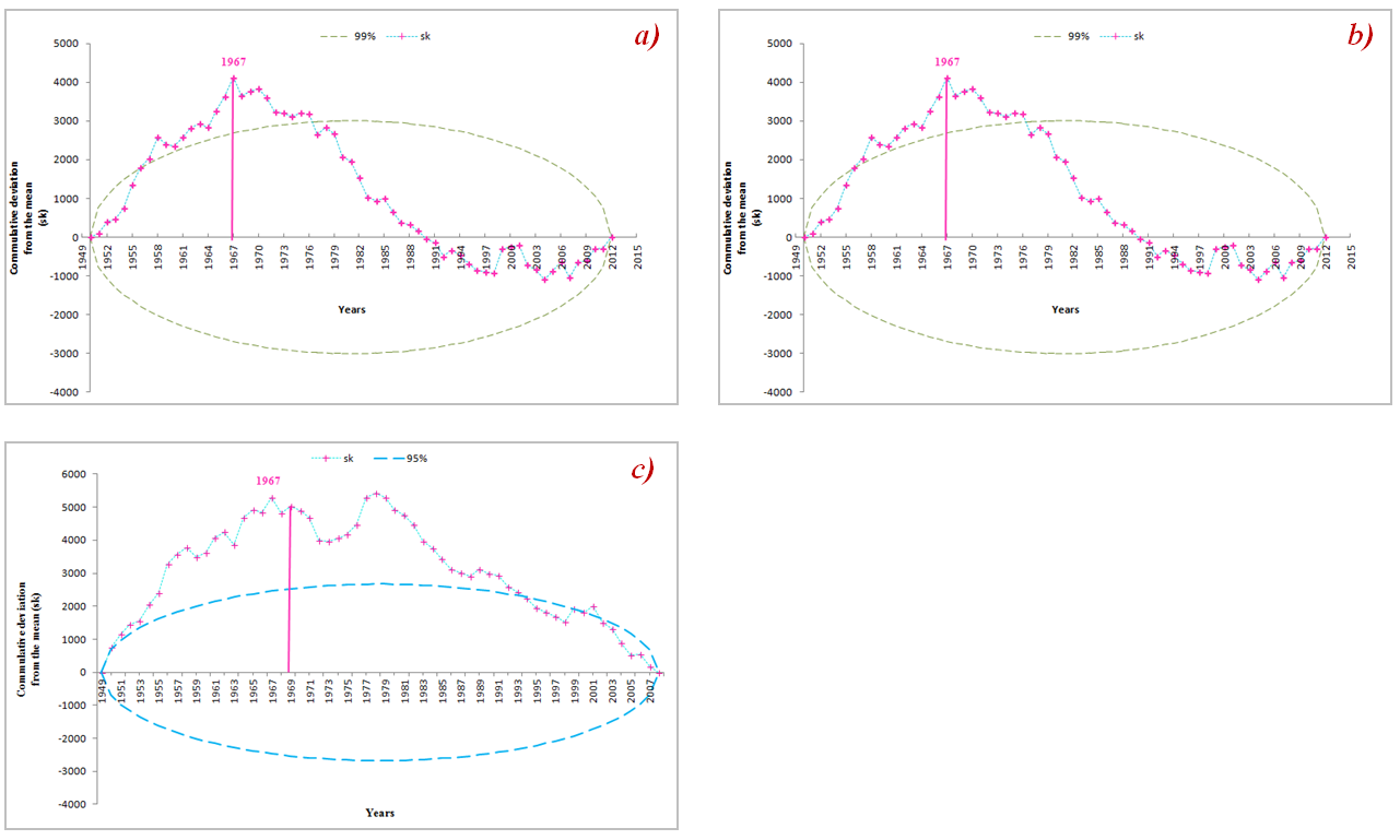 | Figure 7. Buishand diagram: a) at Ziguinchor raingauge, b) at Bignona raingauge, c) at Oussouye raingauge |
5. Conclusions
- This paper aims to highlight rainfall variability at yearly scale and identify the various climate situations and characteristics in the lower valley of the Casamance river basin. To reach our objective, we have proceeded through some analysis based on statistical test of randomness (Autocorrelogram and correlation test of Rank) and rupture (Pettitt, Hubert, Buishand and Lee and Heghinian test), while using the Khronostat software at significance level of 95%. Data of Ziguinchor (1951 to 2012), Bignona (1950 to 2012) and Oussouye (1950 to 2008) rain gauges have been selected for this purpose. Test of randomness show that Time series are random for the stations. Tests of homogeneity evoke the presence of a downward break in the time series of the 3 stations. The probability of this break is more pronounced for Ziguinchor than successively for Bignona and Oussouye. The remarkable fact is that all tests indicate the same date of rupture corresponding 1967. This study provides useful information to climate experts and water stakeholders in understanding the link between climate instability and water availability, thus contributing to the sustainable management of water resources. However, it is important to keep in mind that the analysis presented is only focused on precipitation whereas it is not the only key parameter of the climate. It is also important to recognize the limitations of the Khronostat model. This software does not take into account the existence of gaps within the series to be analyzed. In the future, it would be interesting to find a model that is careless of gaps if we know that in Africa it is very common to have incomplete data. This model should be applied to rainfall, temperature and runoff to determinate relationships between the three, highlight causes of high and low flows, frequency, trends). Statistical analysis on probabibility of occurrence of dry or wet spells to better evaluate possible changes in water resources availability could also be an asset for the considered region.
ACKNOWLEDGEMENTS
- The authors wish to thank the National Agency of Civil Aviation and Meteorology (ANACIM) for their determining support through putting reliable data at our disposal within the framework of this study.