-
Paper Information
- Next Paper
- Paper Submission
-
Journal Information
- About This Journal
- Editorial Board
- Current Issue
- Archive
- Author Guidelines
- Contact Us
World Environment
p-ISSN: 2163-1573 e-ISSN: 2163-1581
2016; 6(3): 79-83
doi:10.5923/j.env.20160603.02

Analysis, Evaluation and Stochastic Modeling of Emission Levels of Three Greenhouse Gases (CO2, H2O and SO2) through Vehicular Activities within Enugu Metropolis
 Abstract
 Reference
 Full-Text PDF
 Full-text HTML
Ezeh Ernest1, Okeke Onyeka2, Nwosu David3, Umeh Joel4
1Chemical Engineering Department, Nnamdi Azikiwe University, Awka, Nigeria
2Plastic Production Section, Scientific Equipment Development Institute, Enugu, Nigeria
3General Laboratory, Scientific Equipment Development Institute, Enugu, Nigeria
4Electroplating Section, Scientific equipment Development Institute, Enugu, Nigeria
Correspondence to: Okeke Onyeka, Plastic Production Section, Scientific Equipment Development Institute, Enugu, Nigeria.
| Email: |  |
Copyright © 2016 Scientific & Academic Publishing. All Rights Reserved.
This work is licensed under the Creative Commons Attribution International License (CC BY).
http://creativecommons.org/licenses/by/4.0/

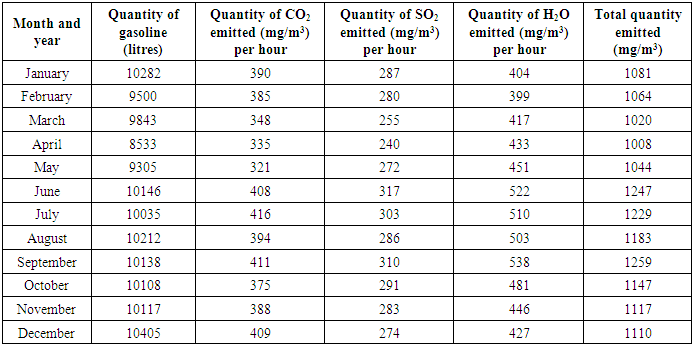
Research was conducted to determine the level of emission of three greenhouse gases (CO2, H2O and SO2) through vehicular activities within Enugu Metropolis using gaseous pollutant sampler envirotech ARM 433 and fourier transform infra-red spectroscopy. The analysis showed that CO2 emission was above the permissible limits of 350mg/m3 in nine out of the 12 calendar month of the study year, 2015. SO2 and H2O were within their respective emission permissible limits across the length of the year studied. Stochastic model equations showed that relative humidity and traffic density greatly influenced the levels of emission of pollutant/greenhouse gases through vehicular activities in any given environment. Stochastic modeling equation successfully predicted the level of gaseous emissions in 2017 within Enugu metropolis which could be adopted by relevant government agencies towards pollution control measures.
Keywords: Stochastic modeling, Greenhouse gases, Pollution and meteorological data
Cite this paper: Ezeh Ernest, Okeke Onyeka, Nwosu David, Umeh Joel, Analysis, Evaluation and Stochastic Modeling of Emission Levels of Three Greenhouse Gases (CO2, H2O and SO2) through Vehicular Activities within Enugu Metropolis, World Environment, Vol. 6 No. 3, 2016, pp. 79-83. doi: 10.5923/j.env.20160603.02.
1. Introduction
- Clean air is essential for good health of humans, animals and birds [2]. Since the industrial revolution, the quality of the air we breathe has deteriorated considerably mainly as a result of human activities [16]. All the countries in the world are facing a common problem of air pollution. Rising industrial production and dramatic rise in traffic on our roads all contribute to air pollution in our towns and cities. This in turn can lead to serious health problems to living things when the air pollution exceeds permissible limits [17]. Pollution is an undesirable change in the physical, chemical or biological characteristics of air, water and soil that has potential health hazard to any living organism particularly man [4]. Any substance that causes pollution is called a pollutant. A pollutant may include any chemical or agrochemical substance, biotic component or its product or physical factor (heat) that is released by man into the environment that may have adverse harmful or unpleasant effects [4]. Pollutants are residues of the things we make use of and throw away. Air pollution is a deliberate or inadvertent deposition of materials in pure air, which affects the physical and/or chemical properties of the air and subsequently, caused detectable deterioration of air quality [11]. Thus polluted air is one which in addition to its normal constituents contains other substances called pollutants. Air pollution has three components; the emitting source, atmospheric transport and dispersal and the receptor [14]. The degree of air pollution depends on the interaction of these identified components. Air pollution results mainly from gaseous emissions of industry, thermal power stations, automobiles, domestic combustions, smoke from fire, burning coal mines, decaying vegetation, volcanic eruption, sewers and smelting industries [1]. The main air pollutants emitted from these different sources include: carbon components (CO and CO2), Sulphur compounds (SO2 and H2S) nitrogen oxides (NO, NO2 and HNO3) and Ozone e.t.c.According to the World Health Organisation [18], millions of untimely deaths are occurring due to the urban air pollution created from burning of solid fuel. Most of the deaths due to air pollution are from developing nations [13]. Usually, children are the most susceptible to harmful influences due to their tender tissues, higher surface volume ratio and relative inhalation rate for healthier growth and build-up [12]. Other effects air pollutants include, greenhouse effects, global warming, acid-rain, eye-irritation, breathe difficulties, genetic abnormalities, blood poisoning, heart diseases, damage to fruits and vegetables and blackening and corrosion of building materials [9].Air pollution control involves a number of measures which include, treatment of industrial wastes before disposal by industries, enlightenment of citizens through different media on the dangers of indiscriminate disposal of waste materials, regular maintenance of vehicles to ensure complete combustion of petrol and construction of motor parks in every nook and cranny of the society to reduce traffic jams which could lead to increased pollution from exhaust fumes of vehicles [7]. On the other hand, air pollution control involves an inter play of issues and interests that are dealt with on daily basis. Many issues involved in air pollution control are mobile sources, cost benefit-ratios in control enterprise and the complimentary efforts of regulatory agencies.Control techniques for limiting pollutant formation and emission include system enclosure, emission capture, products reformations and feed stock modifications e.t.c. [15]. In principle the emission level air quality problem could be resolved with the use of a reliable, fully validated mathematical model based on fundamental description of atmospheric transport and chemical process [10]. The model involves emission patterns, metrology, chemical transformations and removal processes. The efficient management of air resource means the ability to translate a specified time and location pattern of discharges of gaseous residuals into the resulting time and space pattern of ambient concentrations, including consideration of synergistic effects and chemical and physical reactions in the atmosphere after discharge [3]. This translation reflects mostly the impact of various meteorological processes on the transportation and dilution of pollutants in the atmosphere. A host of mathematical and decision support techniques have been developed and employed to aid in forming air-quality planning optimization models. The first category examines deterministic models in which parameters are assured to be known with certainty in advance. In the late seventies and eighties, researchers began to recognize short comings in deterministic models. This led to stochastic approaches that mainly deal with great variability in meteorological conditions [8]. Hence the stochastic approach which accounts for the uncertainties in the parameters. Stochastic models are based on the analysis of past and present data and consist of the observed relationship between variables describing ambient air quality and variable describing the pollution source.This research aims to assess the pollution level of the greenhouse gases (CO2, SO2 and H2O) through vehicular emission in Enugu Metropolis. The objectives are to employ stochastic model in relation to understanding variables that precipitates persistent presence of greenhouse gases in our environment and predict the future emission levels with a view to formulating air pollution control policy.
2. Materials and Methods
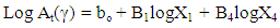
- The meteorological data (traffic density, wind speed, dry-bulb temperature and relative humidity were obtained from Enugu State University of Science and Technology, meteorological observation. The quantity of gasoline (litres) consumed per hour was obtained through questionnaire analysis.The quantity of CO2, H2O and SO2 emitted through vehicular emission was obtained and analysed using gaseous pollutant sampler environtech ARM 433 and Fourier – transform infra-red spectroscopy [13]. This is an independent instrument used for monitoring and quantifying gaseous pollutants like SO2, COx, H2S etc, in ambient condition using chemical methods. Sampled is bubbled through reagents that absorb specific gaseous pollutants and absorbing media analyzed. Analysis: The data obtained were subjected to analysis of variance and regression at 99% confidence level.The model: Level emission
 | (1) |
 | (2) |
 | (3) |
3. Results and Discussion
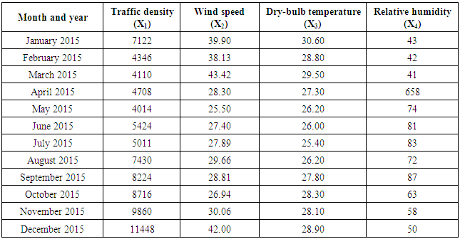
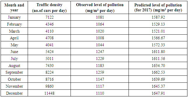
- X1 = Traffic density; X2 = Wind speed; X3 = Dry-bulb temperature; X4 = Relative humidity. Table 1 shows that the months of September to December, 2015 witnessed the highest traffic density in the metropolis which could be due to approach and celebration of yuletide season, while the lowest traffic density was recorded in the months of February, March and May.
|
|
|
4. Conclusions
- The study showed that factors like traffic density and relative humidity can greatly influence the level of emission of pollutant/greenhouse gases especially through vehicular activities at any time in any environment which were validated using stochastic model equation. Stochastic model equation was used to predict the level of emission of greenhouse/pollutant gases for 2017 and the prediction revealed increase in level of emission by over 60%. The consequence of this development to man and his ecosystem should be unpleasant. Policy makers across every government level could adopt this model approach in coming up with strategies that will control and regulate the level of emission of pollutant gases to the environment.