Afrifa-Yamoah E. 1, Bashiru I. I. Saeed 2, Azumah Karim 3
1Graduate Studies, Kwame Nkrumah Univ. of Science Technology, Kumasi, Ghana
2Mathematics and Statistics Department, Kumasi Polytechnic, Ghana
3Al-Huda Islamic School, Kumasi, Ghana
Correspondence to: Afrifa-Yamoah E. , Graduate Studies, Kwame Nkrumah Univ. of Science Technology, Kumasi, Ghana.
| Email: |  |
Copyright © 2016 Scientific & Academic Publishing. All Rights Reserved.
This work is licensed under the Creative Commons Attribution International License (CC BY).
http://creativecommons.org/licenses/by/4.0/

Abstract
Statistical modelling and data analysis is a crucial instrument in understanding rainfall processes. This article aims at examining the rainfall pattern and fit a suitable model for rainfall prediction in the Brong Ahafo (BA) Region of Ghana. Data from 1975 to 2009 were collected from the Department of Meteorology and Climatology in the BA region. The results revealed that the region experience much rainfall in the months of September and October, and least amount of rainfall in the months of January, December and February. SARIMA (0,0,0)×(1,1,1)12, with an AIC score of 8.985894, has been identified as an appropriate model for predicting monthly average rainfall figures for the Brong Ahafo Region of Ghana and hope that when adopted by the Ghana Metrological Agency and other relevant governmental organisations like the National Disaster Management Organisation (NADMO), it will in the long run help in accurate forecasting and education of the populace on rainfall expectancies.
Keywords:
Statistical modelling, Forecast, Decision making, Brong Ahafo, Ghana
Cite this paper: Afrifa-Yamoah E. , Bashiru I. I. Saeed , Azumah Karim , Sarima Modelling and Forecasting of Monthly Rainfall in the Brong Ahafo Region of Ghana, World Environment, Vol. 6 No. 1, 2016, pp. 1-9. doi: 10.5923/j.env.20160601.01.
1. Introduction
Natural resource management is heavily driven by climate. Far reaching impacts of climate change are being felt in ecological, resource-degradation and hydrological process in Ghana. A typical example in Ghana is the constant decrease in the water levels of the Akosombo Hydropower Generation Dam, which is the main source of power generation thus the persistent “dumsor”. The changing climatic conditions have immensely affected rainfall patterns in Ghana, recording downward figures since 1993, which, Kwamena & Benneh (1995) attributed it to the activities of the over 70% citizenry direct or indirect involvement in rain dependencies agriculture. The Forestry Commission of Ghana estimated 8.2 million hectares of forest in 1990 reduced to 1.2 million hectares in 1997 as a result of illegal logging, overgrazing, bad mining practices, industrialization, environmental pollution and urbanization. The irony of the situation is that Ghana is a rain dependent agricultural country. Amidst this background however, flood and rainstorm have been identified under hydro-meteorological disasters in Ghana’s disaster profile for which technical committees have been tasked to develop various hazard maps and to draw education and training programme, emergency preparedness and response plans and advice for the government and major stakeholders (NADMO, 2015). The BA Region has had its fair share of flood. In 1999, the northern part of BA Region was among the victims of the “northern floods” in which over three thousand persons were affected. The flood re-occurred in 2007 and affected over three hundred thousand (307,127) persons (NADMO, 2015). A major shortfall in disaster management in developing countries, like Ghana, is the limited capacity of responsible agencies to issue correct and up-to-date happenings of events to the populace. This has resulted in deaths and loses of valuable properties that could have been saved. To complement the efforts of these technical committees, resourced materials must be made available. There is the need for appropriate modelling, if possible, of relevant events of life to adequately inform decision making processes, thus the need for this study. Several studies on climatic conditions have been undertaken to understand and identify the changing trend in temperature, rainfall, humility and other related conditions with temperature studies have witnessed consistent agreement in results among researchers (Chin (1977); Coe (1982); Cowpertwait (1994); Chandler (1997); Dunn (2004); Carmona (2005): Beatrice et al (2014); R.C. Noven et al (2015)). However, rainfall studies have resulted in diverse results in same spatial area. A typical case in literature is the study in the Meditarranean, researchers have reported diverse variability patterns (Maheras (1988), Maheras & Vafiaris (1990), Benifo, Orellara & Zunta (1994). In Ghana, climate studies have been conducted and reported in literature. Several attempts have been made by researchers to formulate models that best predict rainfall figures in the country. Abdul-Azziz et al (2013) found a significant change in rainfall pattern over time in the Ashanti Region of Ghana and proposed a SARIMA (0,0,0)×(2,1,0)12 with a BIC score of 8.592 as the best model for forecasting the rainfall figures for the region. Similar studies in the New Juaben Municipality of the Easten region of Ghana reported a SARIMA (0,0,1)×(1,1,1)12 model with BIC of 8.077 as the most efficient model for forecast rainfall figures in this part of the country (Ampaw, Akuffo, Opoku & Lartey, 2013). Wiredu, Nasiru & Asamoah (2013) also reported SARIMA (0,0,1)×(0,1,1)12 with AIC of 591.03 as the best model for forecasting rainfall figure in the Navrongo Municipality of Ghana. The current study seeks to statistically investigate the rainfall pattern in the Brong Ahafo Region of Ghana.
2. The Study Area
The Brong Ahafo (BA) region is the second largest region in Ghana with a land area of 39,558 km2 with 22 administrative districts and municipalities. It covers 16.6% of the country’s total land area located within longitude 0° 15’ E-3° W and Latitude 8° 45’ N-7° 30’ S in the west central part of Ghana. Stretching across the center of the country, the Region enjoys a heavy to moderate amount of rainfall. Generally, there is a gradual decrease of rainfall from the south where the average annual rainfall is well over 1651mm (65 inches). To the north of Berekum along the western border of the Region, the average annual rainfall is about 1,143-1,270mm i.e. (45-50 inches). Rainfall in the northern parts of the Region is, however quite low. The average annual total rainfall of the Region is 1,088mm – 1,197mm. Rainfall ranges, from an average of 1000mm millimeters in the northern parts to 1400 millimeters in the southern parts. Major rains occur between April and July with the minor falling between September and October. There is a short dry spell in mid-August before the prolonged dry season between November and March. The main farming activities (planting season) starts with the onset of the major seasons rains. The rainfall pattern between 2001 and 2010 indicate an average of 1,280mm and a thirty (30-year) average of 1,244mm reflecting a percentage change of 0.5% between an average of 30 years and 2010. Comparative rainfall figures between 2009 and 2010 reflected 8.9% increase in volume of rainfall (Ministry of Food and Agriculture, 2014).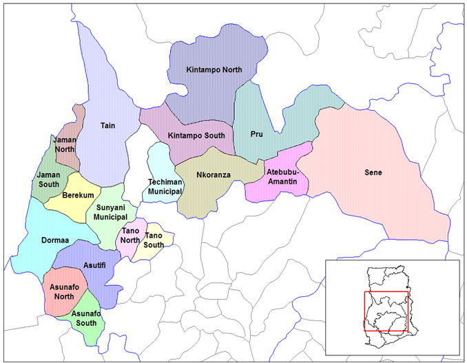 | Map 1 |
3. Methods and Materials
Time series modelling of time spaced events are formulated to understand generation mechanisms of events, forecasting or predicting of future events and also for optimal control of events.
3.1. Box Jenkins Algorithm
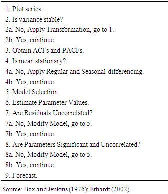
The approach is to use data in the past to provide forecasts. Using the ARIMA self-projecting time series forecasting model, we hope to find a mathematical formula that will approximately generate the historical patterns in a time series. The self-projecting time series uses only the time series data of the activity to be used to generate forecasts. This approach is typically useful for short to medium-term forecasting (Erhardt, 2002). The underlying goal of the Box-Jenkins Forecasting Method is to find an appropriate formula so that the residuals are as small as possible and exhibit no pattern. The model-building process involves four steps, repeated as necessary, to end up with a specific formula that replicates the patterns in the series as closely as possible and also produces accurate forecasts. This process is outlined in Table 1.Table 1. Box-Jenkins Modelling Algorithm
 |
| |
|
3.2. Stationarity and Non-stationarity
The stationarity of the n-th order time series is established if | (1.1) |
for all 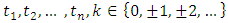 and all
  This implies that the joint distribution is invariant to time shift by k for all n = 1,2,.... (1.1) depicts a time series as strictly stationary. The converse is true for non-stationary. If (1.1) is true for
  it is also true for
  because the m-th order distribution function determines all distribution functions of lower, hence a high order of stationarity always implies a lower order of stationarity (Wei, 2006). Mostly, a weaker sense of stationarity is defined in theory and practice. A process is said to be n-th order weakly stationary if all its joint moments up to order n exist and are time invariant. Stationarity plays a crucial role in time series analysis. One can test the stationarity or otherwise of a time series data using the unit root test proposed by Dickey and Fuller in 1979, for testing the hypothesis below;
 If the ADF test statistic is less than the critical value, we fail to accept H0. The test is based on the fact that for stationarity to exist, the roots of the characteristics polynomial of the time series must lie outside a unit circle.
3.3. Model Types
3.3.1. Autoregressive Models of Order p [AR(p)]
The p-th order autoregressive process is given by; | (2) |
with auto-covariance function, | (3) |
and a recursive relation for the autocorrelation function, | (4) |
The process is stationary if the roots of 
 lie outside a unit circle. The pacf vanishes after lag p.
3.3.2. Moving Average Process of Order q [MA(q)]
The q-th order moving average process is | (5) |
The MA(q) process is always stationary because 
 The process is invertible if the roots of
  lie outside a unit circle.The auto-covariance function is given by
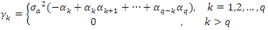 | (6) |
Therefore, the autocorrelation function becomes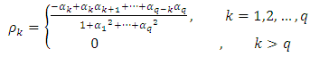 | (7) |
The autocorrelation function of an MA(q) process cuts off after lag q.
3.3.3. Autoregressive Moving Average (p,q) Process
Let,
 A zero-mean ARMA(p,q) process is then defined as,
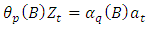 | (8) |
The process is invertible and stationary if the roots of 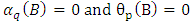 respectively lie outside the unit circle.For
  we get an auto-covariance function of
 | (9) |
and an autocorrelation function of  | (10) |
3.3.4. Autoregressive Integrated Moving Average (p,d,q) Process
A time seires  is said to be homogeneous non-stationarity if
  is stationary for some value of
  A stationary ARMA(p,q) model for
  is given by
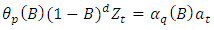 | (11) |
Equation (11) is called autoregressive integrated moving average model, ARIMA(p,d,q).
3.3.5. Seasonal ARIMA (SARIMA) Models
SARIMA models are an adaptation of autoregressive integrated moving average (ARIMA) models to specifically fit seasonal time series. That is, their construction takes into consideration the underlying seasonal nature of the series to be modelled. Many authors have written on SARIMA models extensively. A few amongst them are Box and Jenkins (1976) who proposed them, Priestley (1981), Madsen (2008), Gerolimetto (2010) and Suhartono (2011). A multiplicative seasonal ARIMA model is given by; | (12) |
where 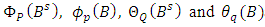 are defined as;
 | (13) |
 | (14) |
where 
 | (15) |
where 
 | (16) |
where s is an integer strictly larger than one (the period),  and
and  Note that
4. Findings and Discussions
In this section, outputs from data exploration and employing the Box-Jenkins Algorithm in building a model are presented and discussed. The data employed in this study were collected from the Department of Meteorology and Climatology in the BA Region, and represent the monthly rainfall figures from January 1975 through December 2009. The data was used since it is a time series data and the observations were collected sequentially in time (monthly). Data was analysed with R. The 420 data points for the time period observed are presented in Figure 2.
4.1. Preliminary Data Analysis
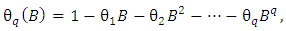
An exploratory routine was employed to reveal some important features in the data set. Figure 1 presents the boxplots of the monthly rainfall figures from 1975 to 2009. | Figure 1. Boxplot of the monthly rainfall figures from Jan. 1975 to Dec. 2009 |
The data considered on monthly basis has some outliers. However, the data look stationary by observation from Figure 2. The month of September recorded the highest amount of rainfall, followed closely by October, which had the highest upper quartile value. The months of January, December and February recorded the least amount of rainfall.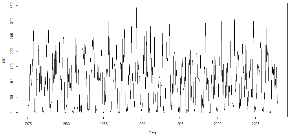 | Figure 2. Time Series plot for Monthly rainfall figures from Jan. 1975 to Dec. 2009 |
The time series plot for the amount of rainfall recorded for the Brong Ahafo from January 1975 to December, 2009 is presented in Figure 2. The regular pattern of up and down is an indication of seasonality. Figure 3 was further investigated by decomposing it into the various components. The decomposed plots of the various components of the time series plot in Figure 2 is as presented in Figure 3.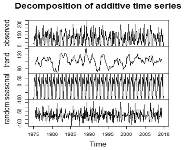 | Figure 3. Decomposed Time Series plot for Monthly Rainfall figures from Jan. 1975 to Dec. 2009 |
From Figure 3, the data have seasonal effect, with a usual rise and fall pattern being experienced yearly over the period. This implies that regular monthly rainfall figures recorded each year was influenced by the rise and fall pattern of the seasonality component. However, the trend seems to be very constant over time, although there are a few ups and downs over some periods. The random effect is very stable over the time period, although one could be interest in its erratic nature between 2007 and 2009.
4.2. Stationarity Test
A formal statistical test is performed at this stage to ascertain the stationarity or otherwise of the data. The hypotheses under consideration are;H0: The data is stationary vrs H1: The data is explosiveThe Augmented Dickey-Fuller test reported a test value of -3.493 and a p-value of 0.9567. This result presents evidence in favour of the null hypothesis, postulating that the data is stationary.
4.3. Model Identification and Fit
The data was divided into two sets, training and test data. Data from January 1975 to December, 2007 were used as training data whiles rest of the data were used as test data for consistency and reliability of our model. The sample autocorrelation function (acf) and partial autocorrelation function (pacf) were examined in Figure 4.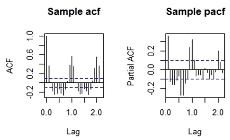 | Figure 4. ACF and PACF plots for the monthly Rainfall figures from January 1975 to December 2007 |
There is a slow decay of the acf and pacf at multiple lags of 12, which are significant. This supports the earlier assertion of seasonality in the data, hence, the need for seasonal differencing with period of 12. The seasonally differenced data is stationary by observing Figure 5.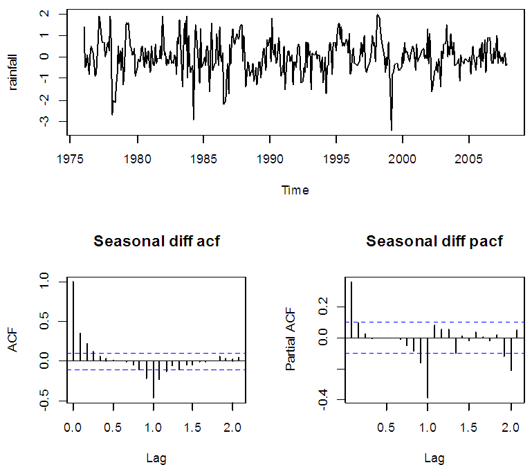 | Figure 5. Time Series, acf and pacf plots for the Seasonally Differenced Rainfall figures from January 1975 to December 2007 |
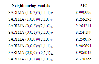
From Figure 5, a spike at 12 in the acf is significant but no other is significant at lags multiple of 12, the pacf shows an exponential decay in the seasonal lags; that is 12, 24, 36 etc. Thus, the seasonal part of the model has a moving average term of order 1 and an autoregressive term of 1. For the non-seasonal part, the acf tails off after lag 2 and the pacf cuts off after lag 1. Therefore, the non-seasonal part has an autoregressive term of 1 and a moving average term of 2. Based on the features portrayed by the plots, an initial SARIMA (1,0,2)×(1,1,1)12 model is proposed. Further investigation of neighbouring models was conducted and the result is as shown in Table 2. Table 2. AIC scores for neighbouring models
 |
| |
|
The best model for the data is SARIMA (0,0,0)×(1,1,1)12 with an AIC score of 8.985894.
4.4. Model Parameters and Verification
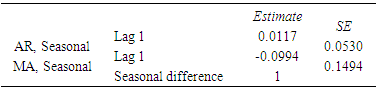
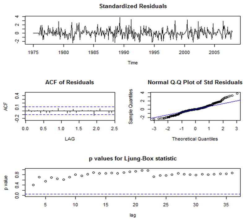
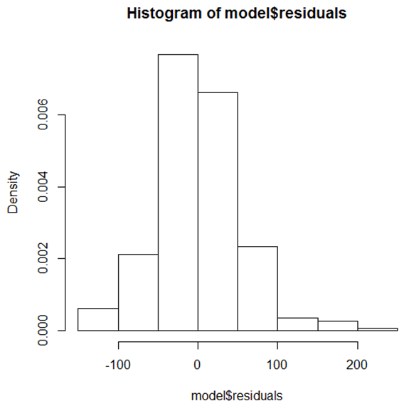
The model parameters are significant from Table 3. The residual plots in Figure 6 suggest that the distribution of the residuals of our proposed model is Gaussian (white noise). This is clearly seen in Figure 7. Hence, our proposed model is justified.Table 3. Parameter estimates of SARIMA (0,0,0)×(1,1,1)12
 |
| |
|
 | Figure 6. Residuals plots for SARIMA (0,0,0)×(1,1,1)12 |
 | Figure 7. Distribution of the residuals of SARIMA (0,0,0)×(1,1,1)12 |
4.5. Forecasting
From Figure 8, the predictive power of SARIMA (0,0,0)×(1,1,1)12 is very appreciable as it fits well to the test data. With exception of the observed value of May 2008 which lied outside the 95% confidence interval, all the other points lie within the confidence interval. The forecasted figures tend to be very close to the actual points. The model predicts well.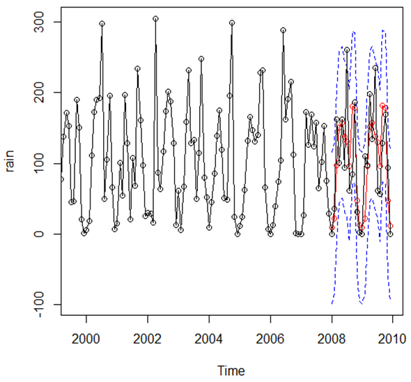 | Figure 8. Prediction of SARIMA (0,0,0)×(1,1,1)12 is shown in red line and dots compared to the test dataset of January 2008 to December 2009 in black line and dots. The 95% confidence interval is overlaid in the blue dotted lines |
5. Conclusions
The region experience much rainfall in the months of September and October, least amount of rainfall in the months of January, December and February. SARIMA (0,0,0)×(1,1,1)12 has been identified as an appropriate model for predicting monthly average rainfall figures for the Brong Ahafo Region of Ghana and hope that when adopted by the Ghana Metrological Agency and other relevant governmental organisations like the National Disaster Management Organisation (NADMO), it will in the long run help in accurate forecasting and education of the populace on rainfall expectancies.
References
| [1] | Abdul-Aziz, A.R., Anokye, M., Kwame, A., Munyakazi, L & Nsowah-Nuamah, N.N.N (2013) Modeling and Forecasting Rainfall Pattern in Ghana as a Seasonal Arima Process: The Case of Ashanti Region, International Journal of Humanities and Social Sciences, 3(3), 224-233. |
| [2] | Ampaw, E. M., Akuffo, B., Opoku, L.S., & Lartey, S. (2013). Time Series modeling of rainfall in New Juaben Municipality of the Eastern Region of Ghana, Contemporary Research in Business and Social Sciences, 4(8), 116-129. |
| [3] | Beatrice, C.B., Nasser, R. Afshar, Selami, O.S. & Fahmi, H (2014) Application of Mathematical Modelling in Rainfall forcast: A Case study of SGS Sarawak Basin, International Journal of Research in Engineering and Technology. 03(11), 316-319. |
| [4] | Benito, Orellana, and Zurita (1994): Análisis de la estabilidad temporal de los patrones de precipitación en la Península Ibérica, in PITA and AGUILAR (Ed): "Cambios y variaciones climáticas en España", Publicaciones de la Universidad de Sevilla, pp183-193. |
| [5] | Box, G. E. P. & Jenkins, G. M. (1976). Time Series Analysis, Forecasting and Control, San Francisco: HoldenDay. |
| [6] | Carmona, R., Diko, P. (2005) Pricing precipitation based derivatives. Int. J. Theor. Appl. Financ. 08(07), 959–988. |
| [7] | Chandler, R.E. (1997) A spectral method for estimating parameters in rainfall models. Bernoulli 3(3), 301–322. |
| [8] | Chin, E.H. (1977) Modeling daily precipitation occurrence process with Markov Chain. Water Resour. Res. 13(6), 949–956. |
| [9] | Coe, R., Stern, R. (1982) Fitting models to daily rainfall data. J. Appl. Meteorol. 21(7), 1024–1031. |
| [10] | Cowpertwait, P.S.P. (1994) A generalized point process model for rainfall. Proc. R. Soc. A Math. Phys. Eng. Sci. 447(1929), 23–37. |
| [11] | Dunn, P. K. (2004), Occurrence and quantity of precipitation can be modelled simultaneously. Int. J. Climatol., 24: 1231–1239. doi: 10.1002/joc.1063. |
| [12] | Erik Erhardt. 2002. Box-Jenkins Methodology vs Rec.Sport. Unicycling 1999-2001. Available at:http://www.statacumen.com/pub/proj/WPI/Erhardt_Erik_tsaproj.pdf (accessed 10- August, 2015). |
| [13] | Gerolimetto, M. 2010. ARIMA and SARIMA Models. Available at:www.dst.unive.it/~margherita/TSLecturenotes6.pdf (accessed 14-August, 2015). |
| [14] | Kwamena D., Benneh, G. (1995). A New Geography of Ghana. Longman Group, England. |
| [15] | Madsen, H. 2008. Time Series Analysis, London: Chapman & Hall. |
| [16] | Maheras (1988) Changes in precipitation conditions in the Western Mediterranean over the last century, Journal of Climatology, vol. 8, 179-189. |
| [17] | Maheras and Vafiaris (1990): "Analyse spectrale des séries chronologiques des précipitations en Méditerranée occidentale", Publications de l'AIC, vol. 3, 421-429. |
| [18] | Ministry of Food and Agriculture (2014). Regional Diaries: Brong Ahafo Region of Ghana. Available at: http://www.mofa.gov.gh/site/?page_id=644 (accessed 13- August, 2015). |
| [19] | National Disaserter Management Organization (2015). Ghana’s Disaster Profile. Available at: http://www.nadmo.gov.gh/index.php/ghana-s-disaster-profile (accessed 13-August, 2015). |
| [20] | Priestley, M. B. (1981). Spectral Analysis and Time Series, London: Academic Press. |
| [21] | Ragnhild, C. Noven, Almut. E.D. Veraart & Axel Gandy (2015) A Lévy-driven rainfall model with application to future pricing. AstA Adv. Stat. Anal, Springer, DOI 10.1007/s10182-015-0246-8. |
| [22] | Suhartono. (2011). Time Series Forecasting by using Autoregressive Integrated Moving Average: Subset, Multiplicative or Additive Model. Journal of Mathematics and Statistics, 7(1), 20-27. |
| [23] | Wei, W.W.S. (2006) Time Series analysis; univariate and multivariate method, Pearson Education, Inc. |
| [24] | Wiredu, S., Nasiru, S. & Asamoah, Y. G. (2013). Proposed Seasonal Autoregressive Integrated Moving Average model for Forecasting Rainfall pattern in the Navrongo Municipality of Ghana, Journal of Environment and Earth Science, 3(12), 80-85. |

 Abstract
 Reference
 Full-Text PDF
 Full-text HTML