1. Introduction

Regional Climate Models (RCMs) have been widely applied and well recognized as an essential tool to address scientific issues concerning of climate variability, changes, and impacts at regional–local scales [1-9]. Numerous RCMs have been developed and applied for simulating the present climate in the worldwide locations. The performance of the RCMs to successfully reproduce the observed regional climate characteristics within the last decades was extensively assessed.

Recently, WRF model has been increasingly used as RCM for the most applications of downscaling, climate simulations, and parameterizations studies. In this work, the climate simulation is carried out with the regional climate WRF model version 3.5 (NCAR Weather Research & Forecasting Model, USA) [10]. This work will focus on the accuracy of the WRF model to successfully reproduce the observed regional climate characteristics of temperature and precipitation over a large domain covering most of the African continent, especially North Africa.

Northern Africa is characterized by a Mediterranean climate at the north coast and a large desert area in the south, where temperatures are the hottest [11]. According to global climate projections [12], the already environmentally stressed Middle East and North Africa region will be one of the most prominent climate change hotspots. Substantial decreases in precipitation, especially during the winter season and intense warming, most pronounced during summer, will probably have strong economic and societal impacts in the region [13].

The aim of this work is to examine the capability of the WRF model to simulate temperature and precipitation over North Africa and it’s validation with available observed datasets. In general, this work is the first simulation (temperature and precipitation) of a series of climate simulations over North Africa, the second simulation is a climate dust simulation, and the third is a climate aerosols simulation.

2. Model, Data and Experimental Design

2.1. Regional Climate Model

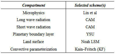
The CLWRF [14] set of modifications, implemented in the version 3.5 of WRF model, was used for the simulations of this study, the WRF model is an advanced mesoscale numerical weather prediction system designed to serve both operational forecasting and atmospheric research needs (http://www.wrfmodel.org). The version 3.5 of WRF model was used for the simulation of this study. The physics options used in this study include the Lin et al. Microphysics scheme [15], Kain–Fritsch convective parameterization scheme [16], CAM Shortwave and Longwave schemes [17], the Yonsei University planetary boundary layer scheme [18], the Noah Land Surface Model (LSM) four-layer soil temperature and moisture model with canopy moisture and snow-cover prediction [19] and MM5 Similarity Surface Layer Scheme [20-24]. A summary of the selected model physics options is given in Table 1. The extent of the North Africa domain is presented in Fig. 1, while the length of the simulation is 5.5 years (July 2006-December 2011), in addition to five months of spin-up time (July-November 2006) which was excluded from our analysis. We have used a horizontal resolution of 50 km and 51 vertical levels. The NCEP/DOE reanalysis-2 dataset was used to provide initial and boundary conditions, and covered the most African continent (including the North Africa interior domain). The output is stored every 6 h (00, 06, 12, 18 UTC) and monthly fields are there from derived. In our study, we evaluate the performance of the WRF model with globally available observations of temperature 2m (Mean T2m, Minimum T2mn, and Maximum T2mx) and precipitation.

Table 1. The model physics options used

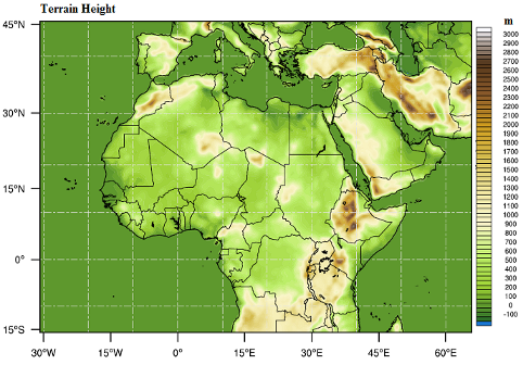Figure 1. Terrain height of model domain over African continent with a 50-km resolution grid

2.2. Data Forcing

The reanalysis data that provide the initial and lateral boundary conditions to the regional climate WRF model in this study is the NCEP/DOE Reanalysis-2 global data [25]. This data was created in cooperation between the National Centers for Environmental Prediction (NCEP) and Department of Energy (DOE). NCEP/DOE Reanalysis-2 is an improved version of the NCEP Reanalysis-1 model that fixed errors and updated parameterizations of physical processes. The NCEP/DOE Reanalysis-2 data are split into 2D and 3D files, the 2D data has T63 horizontal spectral resolution (1.875 × 1.875 degrees) while 3D has horizontal spectral resolution (2.5 × 2.5 degrees), the temporal coverage is 4-times daily and monthly values, and 17 vertical levels, with the top extending to 10 hPa. The global SST data used has weekly of temporal coverage and (1 × 1 degrees) horizontal resolution and updated in the model every 6 hr.

2.3. Observational Datasets

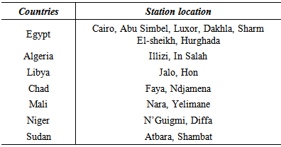
Surface meteorological variables extracted from the model output were compared with the CRU and GPCC gridded datasets and CMORPH from satellite gridded dataset. The Climatic Research Unit Timeseries (CRU TS) datasets contain monthly time series of precipitation, daily maximum and minimum temperatures, cloud cover, and other variables covering Earth's land areas, the CRU version used is CRU TS3.21, 2013 [26] [27] and available through the Climatic Research Unit at the University of East Anglia. The dataset is gridded to 0.5x0.5 degree resolution, based on analysis of over 4000 individual weather station records distributed around the world.

The Global Precipitation Climatology Centre (GPCC) [28] dataset has been established in 1989 on request of the World Meteorological Organization (WMO). It is operated by Deutscher Wetterdienst (DWD, National Meteorological Service of Germany) as a German contribution to the World Climate Research Programme (WCRP). The GPCC’s new global precipitation climatology V.2015 is available in 0.5° x 0.5° resolution based on data from ca. 75,000 stations is used as background climatology for the other GPCC analyses.

The CMORPH (CPC MORPHing technique) produces global precipitation analyses at very high spatial and temporal resolution [29] [30] [31] [32]. This technique uses precipitation estimates that have been derived from low orbiter satellite microwave observations exclusively, and whose features are transported via spatial propagation information that is obtained entirely from geostationary satellite IR data. The CMORPH data has a spatial resolution of 0.5° x 0.5° and 3-hourly temporal resolution.

The comparison focused on mean seasonal of (T2m), maximum (T2mx), minimum (T2mn) temperature and precipitation in order to attribute some of the surface variables biases. Moreover, monthly observations derived from the CRU dataset were used for 18 selected locations over the desert area in North Africa domain for the trends of mean T2m. The choice of stations was based on the hottest places in the domain for the period of interest and the spread of stations across the region. Table 2 shows the stations location in their countries.

Table 2. The 18 stations location in their countries over the study domain

3. Results

In this section the model temperature outputs are compared with the CRU observation dataset while the precipitation is compared with CRU, GPCC and CMPRPH datasets for the study period.

3.1. Temperature Fields

3.1.1. Mean Temperature T2m

The mean T2m of the CRU data for the study period is presented in the top left panel of Fig. 2 as a reference, the top right panel for the WRF model and the bottom panel for the bias during the study period. It is clear from the bias map in Fig. 2.c that the cold bias in the model simulation along with the study period was over most African continent while the warm bias was over the Morocco, Northern of Algeria, Chad, Ethiopia and Kenya.

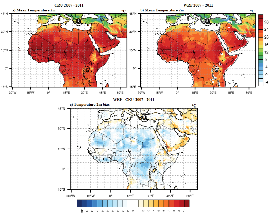Figure 2. The mean T2m temperature of CRU in top left panel (a), WRF in top right panel (b) and the bias map (WRF minus Observations) in bottom panel (c) during the study period (2007-2011)

The simulation bias (WRF minus Observations) is presented in Fig. 3 and the seasonal mean T2m from CRU gridded analysis, as well as WRF simulation during the periods December-January–February (DJF), March-April- May (MAM), June-July–August (JJA) and September- October-November (SON) are shown in Fig. 4, along with the study period.

A first look at the bias maps of T2m for all seasons Fig. 3 shows that the cold bias is dominant in most regions of the model domain. The WRF model simulation has a large cold bias in DJF (Fig. 3a) over northern of Sudan area, moderate in MAM and SON (Fig. 3b, d) especially south of 15° N and the warm bias appears in northern Algeria, Morocco and Ethiopia while in JJA (Fig. 3c) has a small cold bias over the model domain.

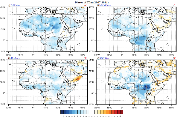Figure 3. The biases (WRF minus observations) of seasonal T2m during the study period (2007-2011)

Fig. 4 shows that the WRF model match with the temperature distribution as in CRU observed data with slightly differences. The WRF model in DJF (Fig. 4b) reproduces the temperature pattern as the same in CRU observations (Fig. 4a) but in the north band the WRF model extends slightly to the south the area over the north band of the domain. In MAM (Fig.4c), the figure shows a band of warm temperature in the Sahel (10°-20° N) along from west to east Africa, this band appears in WRF simulation (Fig. 4d) but with low temperature from the observed data and also the southern band, while CRU and WRF are in good agreement in the northern band. In JJA, the WRF model (Fig. 4f) matches best with the CRU observations (Fig. 4e). They both locate the peaks of high temperature in the Sahara desert. In SON, the WRF model (Fig. 4h) had low temperature compared to CRU observations data (Fig. 4g).

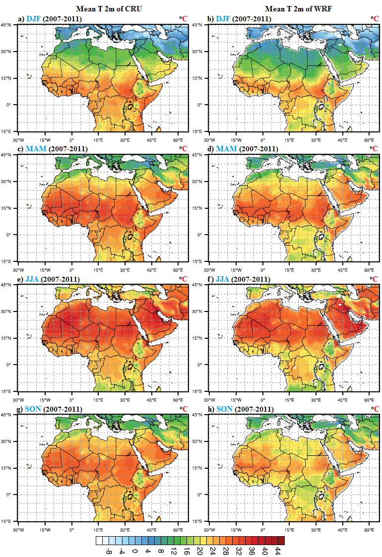Figure 4. The seasonal mean of T2m from CRU gridded analysis in the left panel for (a, c, e and g) and WRF model in the right panel for (b, d, f and h) during the study period (2007-2011)

3.1.2. Stations Comparison

A comparison between WRF model simulation and the CRU observed data was performed over 18 station locations (Table 2) in the desert area (hottest area) over the study domain. The closest model land grid point to the stations coordinates is considered with the mean T2m of the closest CRU grid point for the comparisons. As shown in Figs. 5, 6 and 7, the 18 stations divided over 7 countries, Fig. 5 represent six stations over Egypt due to importance of this area in the second simulation (dust simulation), Fig. 6 has two stations over Algeria, two stations over Chad and two stations over Libya, Fig. 7 has two stations over Mali, two stations over Niger and the last two over the Sudan area.

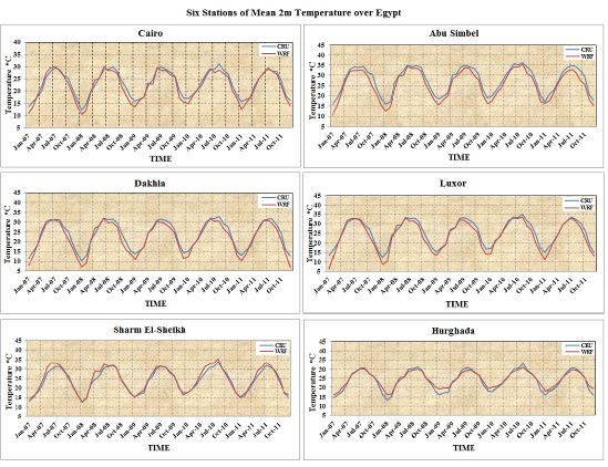Figure 5. The time series of the mean T2m of six stations over Egypt

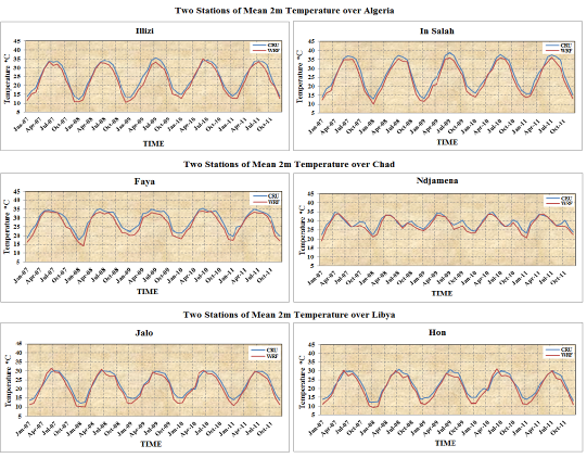Figure 6. The time series of the mean T2m of Two stations for each of the Algeria, Chad and Libya

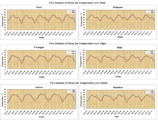Figure 7. The time series of the mean T2m of Two stations for each of the Mali, Niger and Sudan

Overall the WRF model matches best with the peak of maximum values of the T2m for the most of the 18 stations but has slightly low values from the CRU observed data. In general the station location and the nearest grid points in the model may lead to some discrepancies. For most of the cases though, the modeled T2m is closer to the gridded CRU data, which are of the similar horizontal resolution.

3.1.3. Mean Maximum Temperature T2mx

As shown in Fig. 8 for the biases maps, the DJF bias (Fig. 8a) shows strong cold bias over the north band of domain especially over the northern of Sudan area. The MAM bias (Fig. 8b) shows the cold bias appears over the south band of domain, while the warm bias appears in the south coast of Mediterranean sea, the west coast of the Red Sea, Ethiopia, and over the small parts in West Africa. The JJA bias (Fig. 8c) shows the most of cold bias appears over north band of domain, while the warm bias appears over the southern of Morocco and small parts over the south band. The SON bias (Fig. 8d) shows the warm bias appears over the northern of Libya, Algeria and Morocco, while the cold bias is concentrated over the southern of Sudan area.

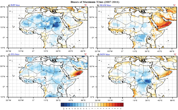Figure 8. The biases (WRF minus observations) of maximum T2mx during the study period (2007-2011)

In DJF, the WRF model (Fig. 9b) captures the main features of T2mx as in CRU data (Fig.9a) but with low temperature over the northern Africa. In MAM, the model (Fig. 9d) matches well with the temperature pattern as appears in CRU data (Fig. 9c) but with slightly low temperature especially over the south band of domain. In JJA, The WRF model (Fig. 9f) captures the temperature distribution as in CRU observations (Fig. 9e) but with slightly low temperature especially over north band of domain. In SON, the WRF model (Fig. 9h) recorded low values of temperature from the CRU observations (Fig. 9g) over the south band of domain, while recorded with slightly low temperature values over the north band.

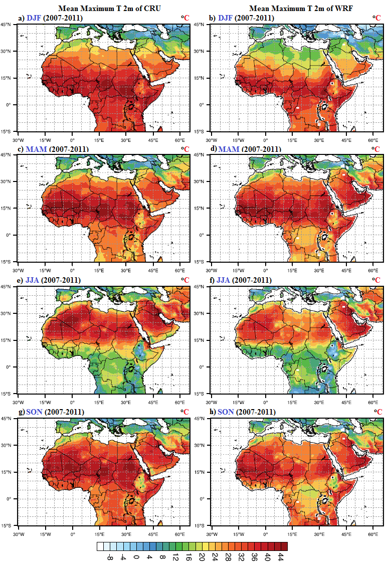Figure 9. The seasonal mean of T2mx from CRU gridded analysis in the left panel for (a, c, e and g) and WRF model in the right panel for (b, d, f and h) during the study period (2007-2011)

3.1.4. Mean Minimum Temperature T2mn

As shown in Fig. 10 for the biases maps, in DJF bias (Fig. 10a) the cold bias appears in north and south bands of the domain, while the warm bias appears in the middle band. In MAM bias (Fig. 10b), the warm bias appears over the north band while the cold bias appears over the south band of the domain. In JJA bias (Fig. 10c), the warm bias appears in the north and south bands of the domain, while the cold bias appears in the middle band. In SON bias (Fig. 10d), the cold bias is located over most Africa continent, while the warm bias over the northern of Algeria, Morocco and Ethiopia.

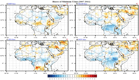Figure 10. The biases (WRF minus observations) of minimum T2mn during the study period (2007-2011)

In general, the WRF model (Fig. 11 b, d, f and h) reproduces well the pattern of the minimum temperature as appears in the CRU observed data (Fig. 11 a, c, e and g). In DJF, the WRF model (Fig. 11b) captures the low temperature over the north band of the domain as the same in CRU data (Fig. 11a), while in the middle band the model recorded higher values of temperature than the observed data. In MAM, the model (Fig. 11d) captures the highest values of temperature in the middle band of the domain as appears in the CRU data (Fig. 11c), while the model recorded slightly higher temperature than the CRU observed data in the north band. In JJA, the WRF model (Fig. 11f) is in good agreement with the CRU observations (Fig. 11e), the WRF model locate the temperature pattern of low and high values. In SON, the WRF model (Fig. 11h) reproduces the temperature pattern as the same in the CRU observations (Fig. 11g) but with slightly low temperature values in the middle band of the domain.

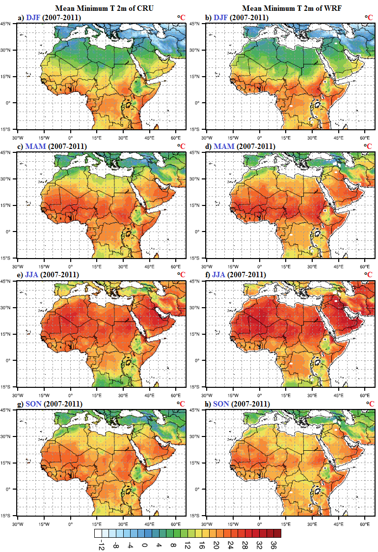Figure 11. The seasonal mean of T2mn from CRU gridded analysis in the left panel for (a, c, e and g) and WRF model in the right panel for (b, d, f and h) during the study period (2007-2011)

3.2. Precipitation Fields

WRF-simulated for the spatial patterns of the seasonal precipitation over the study period are compared to those from CRU, GPCC and CMORPH datasets for DJF in Fig. 12a, b, c and d, JJA in Fig. 12e, f, g and h, MAM in Fig. 13a, b, c and d and SON in Fig. 13e, f, g and h. As most of the African continent lies within the tropics, the seasonal migration of the tropical rainbelt that regulates the alternation of wet and dry seasons is the principal characteristic of precipitation over the Africa continent. Furthermore, small shifts in the position of the rainbelt can result in large local changes in precipitation; this has a direct impact upon water resources and agriculture in the semiarid regions of the continent, such as the Sahel. There are also regions on the northern and southern limits of the continent with winter rainfall regimes that are governed by the passage of mid-latitude fronts. The wettest regions in Africa are those of the equatorial, tropical rainforest climate type, where there is rain throughout the year, with two peak periods corresponding to the double passage of the tropical rainbelt. The driest regions are those of the desert climate type, such as those of the Sahara, Kalahari and Somali deserts, where there is very little precipitation [45].

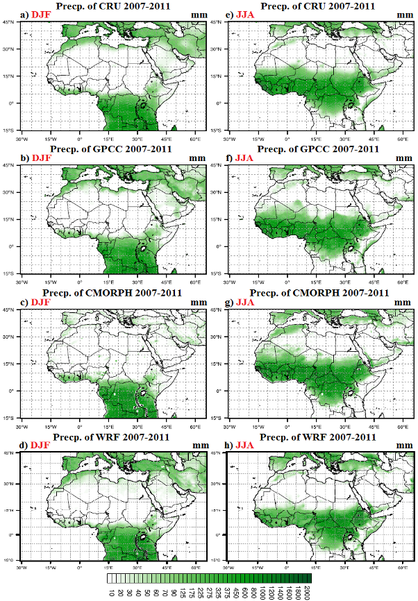Figure 12. The Averaged 2007-2011 precipitation (mm) in left panel from a) CRU, b) GPCC, c) CMORPH and d) WRF for DJF season and in right panel from b) CRU, d) GPCC, f) CMORPH and g) WRF for JJA season

Figure 13. The Averaged 2007-2011 precipitation (mm) in left panel from a) CRU, b) GPCC, c) CMORPH and d) WRF for MAM season and in right panel from b) CRU, d) GPCC, f) CMORPH and g) WRF for SON season

During the study period, the dry North African and Middle East part of the domain is realistically simulated by the WRF model. Over the African continent the main precipitation bands and precipitation patterns are reproduce well with the WRF model as shown in Fig. 13 and Fig. 14. The rain belt and precipitation distributions are well represented by WRF model in DJF and JJA as shown in Fig. 12, left panel and right panel, respectively. The WRF model captures well the precipitation distributions over the south band of the domain, but the intensity was slightly underestimation over the West Africa (Sierra Leone, Liberia, Cote D’Ivoire and Ghana) and was low values over the northern part of the domain. In addition, the WRF shows a heavy rainfall over some orographic area such as Ethiopian highland. In JJA the rain belt in the south band shifted towards the south and the WRF matches with the CRU and GPCC datasets in the northern part while the CMORPH dataset has intensive values of precipitation over Algeria and Atlas Mountains. In general, the three datasets compared to the WRF model have similarities in the precipitation patterns for the study period of comparison especially over the south band of the domain. Yet some differences exist especially over the northern band. For example, there is poorness in the precipitation for CMORPH dataset over the northern band of the domain in DJF season Fig. 12c.

As shown in Fig. 13 for MAM (left panel) and SON (right panel) seasons, in MAM the WRF represented well the precipitation pattern in the northern part but has slightly intensive values over Atlas Mountains and WRF recorded values of precipitation over south east of Algeria as clearly in CMORPH dataset. The WRF recorded underestimation values in the south band especially over the Democratic Republic of Congo, while the WRF recorded overestimation over Uganda, Rwanda and Burundi. In SON, WRF model simulation was closer to the CRU dataset in the northern part especially over Atlas Mountains along with the south coast of the Mediterranean Sea until Tunisia but the GPCC and CMORPH datasets recorded values of precipitation over Algeria, Mauritania and Mali and this situation not exist in CRU dataset. In the south band, the rain belt in the WRF is shifted toward the south reached to south of Sudan. The WRF recorded slightly intensive values of precipitation over Uganda, Rwanda and Burundi, while recorded slightly low values over the Democratic Republic of Congo and WRF was underestimation over West Africa.

In conclusion, the WRF model reproduces well the rain belt and precipitation distributions in DJF and JJA seasons, while was slightly incapability in simulation in MAM and SON.

4. Conclusions and Future Plans

While Numerous RCMs have been developed and applied for simulating the present climate in the worldwide locations, we used the climate version of WRF model to conduct a series of climate simulations over North African domain. These simulations are climate simulation, climate dust simulation, and climate aerosols simulation.

We have presented results of 5.5 years simulation by the WRF model in climate mode. The WRF simulation succeeds in reproducing the main geographical distribution and seasonal variations of temperatures, although some biases are apparent. Model temperature is mostly underestimation from the observational data along with the simulation period. The location and timing of the tropical rain belt is well reproduced, as well as the seasonal precipitation cycle. The apparent of cold biases is due to the overestimation of WRF clouds over the domain of study, where the model has uncertainty in the simulation of clouds.

The future plan including a dust and aerosols simulations, will conduct using WRF model in climate mode for the same period and physics configuration.