Kunio Ueda
Department of Biological Resources Management, School of Environmental Science, The University of Shiga Prefecture, Japan
Correspondence to: Kunio Ueda, Department of Biological Resources Management, School of Environmental Science, The University of Shiga Prefecture, Japan.
| Email: |  |
Copyright © 2012 Scientific & Academic Publishing. All Rights Reserved.
Abstract
Hypoxic conditions are reported in various water bodies throughout the world. However, the mechanisms of hypoxia development have not been analyzed sufficiently. Hypoxia has mainly been researched in field studies, and here laboratory experiments are conducted to examine the relationships among dissolved oxygen (DO), water depth, thermocline development, and microorganism activity. A mathematical equation to express the recovery of DO concentration in a water column was developed and tested against laboratory simulations. From these results, it is expected that shorelines that are natural beaches or that are bays with islands will have superior DO concentrations than will shorelines with vertical seawalls. It is also expected that at greater depths, the sea more easily becomes hypoxic for bottom sediment with the same organic matter content. The rate at which oxygen diffuses from the air to the water is slower than for diffusion within the water column. Diffusion within the water column is slower than the rate at which microorganisms in the bottom sediment consume oxygen, making it impossible for oxygen to be replenished through diffusion in the presence of a pycnocline. Causes of hypoxia observed in various areas of the world, such as Tokyo Bay, Lake Erie, Chesapeake Bay, Black Sea, and Baltic Sea, are discussed in terms of the mechanisms demonstrated here.
Keywords:
Hypoxia, Anoxia, Water Depth, Thermocline, Halocline, Dissolved Oxygen
Cite this paper: Kunio Ueda, Modeling of Dissolved Oxygen Concentration Recovery in Water Bodies and Application to Hypoxic Water Bodies, World Environment, Vol. 3 No. 2, 2013, pp. 52-59. doi: 10.5923/j.env.20130302.03.
1. Introduction
Hypoxia has been observed in many places, including the Gulf of Mexico, Chesapeake Bay, Lake Erie, Baltic Sea, Black Sea, offshore areas of the Changjiang Estuary, Tokyo Bay, Ise Bay, the Ariake Sea and the Seto Inland Sea. Hypoxia is thought to be severely toxic for shellfish and fish. Hypoxia is also considered to develop into anoxia and finally to lead to the development of blue tides, which are observed in Tokyo Bay and Ise Bay in Japan. Blue tides occur in the surface seawater due to the oxidation of hydrogen sulfide produced by sulfate-reducing microorganisms in the seafloor sediment.The amount of gas dissolved in a liquid is described by Henry’s Law, and the main factors that control the dissolution of gasses in a liquid are pressure and temperature. Further, Truesdale et al. developed a model to determine the maximum dissolved oxygen (DO) concentration in water at various temperatures[1]. However, these models are not enough to understand how oxygen dissolves in water and the occurrence of hypoxia in the ocean. Hypoxia is thought to be caused by eutrophication. Eutrophication in bodies of water occurs mainly by the influx of untreated sewage and agricultural runoff. The increased nutrient loads induce phytoplankton blooms, which upon decay, sink to the bottom of the sea. The decomposition of this biomass by microorganisms consumes DO. Therefore, much effort is made to reduce the nutrient effluent from the drainage basin. Currently, sewage treatment is greater than 90% in Tokyo[2] and about 70% in Aichi Prefecture[3]. Farmers have been advised to use fertilizers minimally in cultivating crops. However, areas of hypoxia are spreading and becoming more severe in the nearby water bodies of Tokyo Bay and Ise Bay.There are factors aside from eutrophication that are thought to induce hypoxia. For example, the relationship between dissolved oxygen concentration and microorganism activity should be discussed. The influence of pycnoclines, such as thermoclines and haloclines, on the concentration of DO should also be examined. Here, we examine the effects of these parameters on DO and develop a mathematical model of the development of hypoxia using three experimental setups.
2. Materials and Methods
2.1. Experiment 1: Developing the Model of DO
Plastic pipes with an inner diameter of 70 mm and length of 2000 mm were capped on one end and filled with distilled water to give water depths of 45, 90 and 180 cm. Next, the water column was bubbled with nitrogen gas to force out the oxygen, and DO at the middle layer of the water column was measured using a DO meter with a galvanic cell (HORIBA OM-51). Experiments were carried out at room temperature. DO was measured for 270 h at water depths of 45 and 90 cm and for 1300 h at 180 cm.
2.2. Experiment 2: Influence of Organic Matter
Sand collected from the shore of Lake Biwa at Hikone City, Shiga Prefecture was sieved to collect particles with a diameter of 0.5 to 1.0 mm. Sand (200 g) was well mixed with 0.125 or 0.25 g cellulose powder (particle size is 200 to 300 mesh No., Toyo Roshi Co. Ltd.) and 0.2 g agricultural soil. The soil mixture was placed into the bottom of the plastic pipe and water from Lake Biwa was poured in slowly to give a water depth of 180 cm. The water was collected from the surface of Lake Biwa near Hikone Port in June 2009, and representative chemical properties determined by JIS methods are shown in Table 2. DO was measured every 2 or 3 days. The labels Bottom, Lower, Middle and Upper in Figures 7, 8 and 9 correspond to depths of 170, 140, 90 and 45 cm, respectively as shown in Figure 1.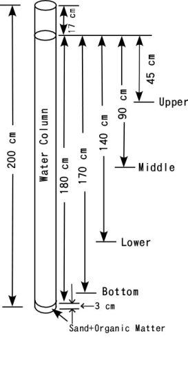 | Figure 1. Schematic of experimental setup for Experiment 2 (influence of organic matter) |
2.3. Experiment 3: Influence of Thermocline
Distilled water (3.4 l) maintained at the room temperature (about 24C) was poured into the same tube as was used in Experiments 1 and 2, giving a water depth of 90 cm. The column was bubbled with nitrogen gas to force out the oxygen. Then 3.4 l of distilled water saturated with oxygen and maintained at 30C was poured on top of the bottom water very quietly. A temperature difference between upper and lower layers was established immediately by pouring in the warmed water. The upper half of the column was covered with an electric blanket and maintained at about 30C. The water temperature was measured by thermometers at 10-cm intervals, and DO concentration was measured using a DO meter at the depths of 170, 140, 60, 20 cm every 2 h for the first 6 h and every 24 h after 6 h. As DO concentration became constant after 3 days, DO was measured every 8 days. A schematic of the experimental setup used in Experiment 3 is shown in Figure 2.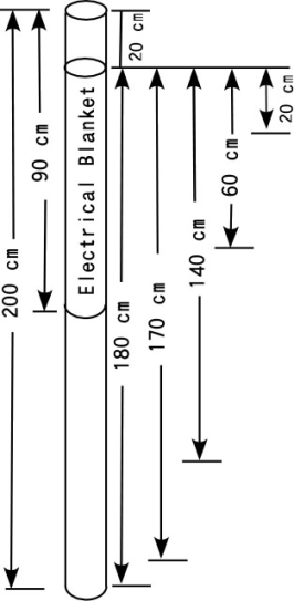 | Figure 2. Schematic of experimental setup for Experiment 3 (influence of thermocline) |
2.4. Tokyo Monitoring Post
The Tokyo Monitoring Post was established about 5 km offshore Chiba Port in Tokyo Bay by the Japan Coast Guard, which continues to measure temperature, salinity, DO, and other parameters and to make the data available to the public via the Internet[4].
3. Results and Discussion
The rate at which DO concentration increases in a body of water is proportional to the surface area of the water column and inversely proportional to the volume of the water column. The difference between the maximum concentration and the present concentration of DO at a given temperature is important in determining the rate at which DO increases. These two aspects are described by Equations (1) and (2), respectively, as  | (1) |
and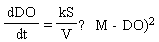 | (2) |
where DO is in mg/L, S is the surface area (cm2), V is the volume (cm3), k is a constant of S/V and M is the maximum DO. dDO/dt is the change in DO concentration in mg/L/h. Equations (1) and (2) were integrated as shown in Equations (3) and (4).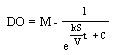 | (3) |
and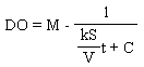 | (4) |
C is the constant of integration. Simulation values generated by Equations (3) and (4) were compared against the measured DO obtained from the experiments. The values generated using Equation (3) coincided with the data of Experiment 1 for the first 100 h, but thereafter, data from Experiment 1 diverged from the values generated by Equation (3) (Figure 3). The data generated using Equation (4) coincided with the results of Experiment 1.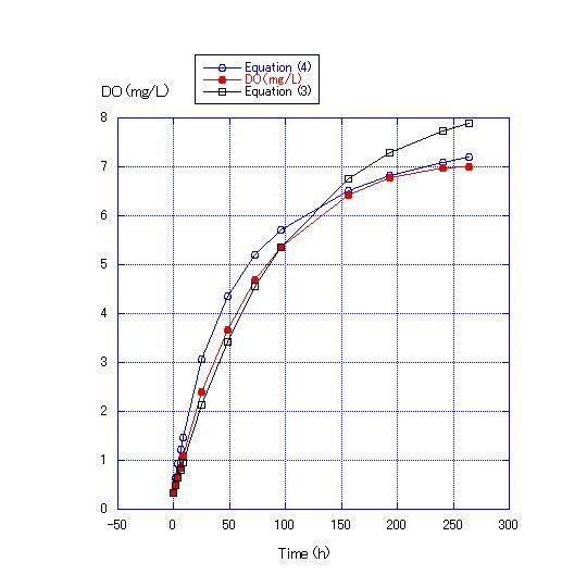 | Figure 3. Comparison of the measured DO concentration for a water depth of 45 cm and the values calculated by Equations (3) and (4). Room temperature was about 22.4C. DO at the start of the experiment was 0.33 mg/L. The C values were determined when t is zero. The values of the kS/V term for Equations (3) and (4) were 1/100 and 1/400, respectively |
In Equation (4), the values of the kS/V term were changed to concrete figures and Equation (4)-1~(4)-6 were obtained. In Figure 4, where the water depth was 45 cm, the values of the kS/V term in Equations (4)-1 and (4) -2 became 1/400 and 1/500, respectively. In Figure 5, where the water depth was 90 cm, the values of the kS/V term in Equations (4)-3 and (4)-4 became 1/900 and 1/1000, respectively. In Figure 6, where the water depth was 180 cm, the values of the kS/V term in Equations (4)-5 and (4)-6 became 1/2500 and 1/3000, respectively (Table 2).V in Equation (4) can be expressed as S*D, where D is water depth. | (5) |
The values of k/D obtained from the kS/V terms of the Equation (4)-1~(4)-6 of Experiment 1 and the ratios of D calculated from k/D in Equation (5) are shown in Table 1. For the water depth of 180 cm, D was 5 to 7.5, a range that is close to the expected value of 4. It is expected that the error originates from the long run time used to generate the data reported in Figure 6. The period of data collection in Figure 6 was about 54 d and that in Figure 4 and 5 was only 11 d.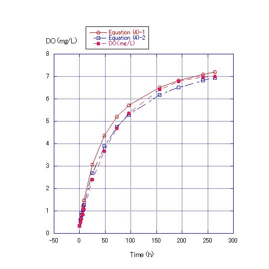 | Figure 4. Comparison of the measured DO concentration for a water depth of 45 cm and the values calculated by Equations (4)-1 and (4)-2. Room temperature was about 22.4C. DO at the start of the experiment was 0.33 mg/L. The values of the kS/V term for Equations (4)-1 and (4)-2 were 1/400 and 1/500, respectively |
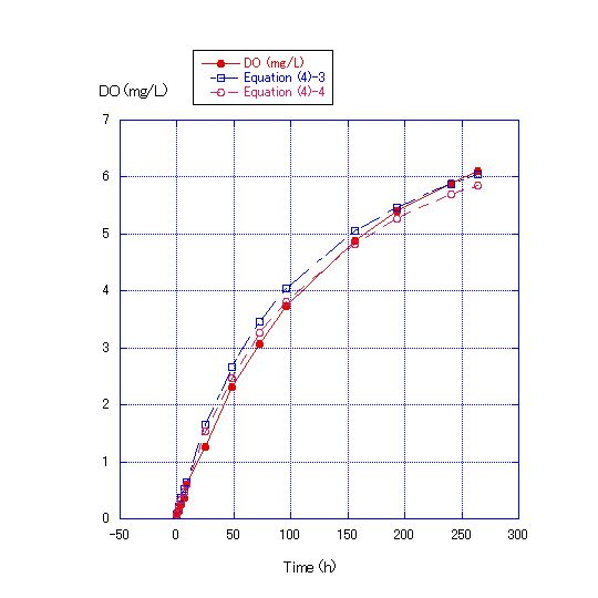 | Figure 5. Comparison of measured DO concentrations for water depth of 90 cm and the values calculated by Equations (4)-3 and (4)-4. Room temperature was about 22.4C. DO at the start of the experiment was 0.07 mg/L. The values of the kS/V term of Equations (4)-3 and (4)-4 were 1/900 and 1/1000, respectively |
| Table 1. Comparison of values for the different water depths |
| | Water depth, D (cm) | Ratio of water depth | k/D obtained in Experiment 1 | Ratio of D | | 45 | 1 | 1/400~1/500 | 1 | | 90 | 2 | 1/900~1/1000 | 1.8~2.5 | | 180 | 4 | 1/2500~1/3000 | 5~7.5 |
|
|
However, for ratios of the water depths of 1, 2 and 4, the ratios of calculated D were 1, 2 and about 4 from Table 1. From Table 1 and Figures 4, 5 and 6, Equation (4) is considered to simulate the DO recovery from zero content in a water column. Based on the calculation of Equation (4), it takes about 10 d for DO to increase to 5 mg/L from zero for a water depth of 0.9 m. Similarly, using Equation (4), it takes about 79 and 154 d for the DO to become 5 mg/L from zero for a water depth of 7.2 and 14.4 m, respectively.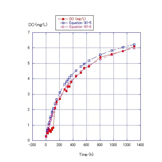 | Figure 6. Comparison of measured DO concentrations for water depth of 180 cm and the values calculated by Equations (4)-5 and (4)-6. The room temperature was from 28.0 to 22.0C. DO at the start of the experiment was 0.26 mg/L. The values of the kS/V term of Equations (4)-5 and (4)-6 were 1/2500 and 1/3000, respectively |
In Figure 6, a column with a water depth of 180 cm was used, and DO was measured at four depths: 45, 90, 140 and 170 cm. Differences in DO among the layers were very small. DO at a depth of 45 cm was the highest of the three layers, but the difference between the top and bottom layers was only 0.4 mg/L after 1300 h. These results show that it is more difficult for oxygen to enter into the water than for it to diffuse in the water column. The rate at which oxygen diffuses in water is greater than that at which oxygen enters into the water. Oxygen that enters into the water diffuses quickly and does not accumulate in the upper layer of the water column.| Table 2. Chemical properties (mg/L) of the surface water used in laboratory experiments |
| | T-P | T-N | COD | BOD | | 0.011 | 0.24 | 2.7 | 0.7 |
|
|
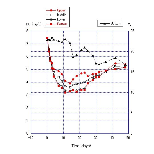 | Figure 7. Transition of dissolved oxygen concentration and bottom temperature for water depth of 180 cm with no addition of cellulose powder to the sand in the bottom soil of the column |
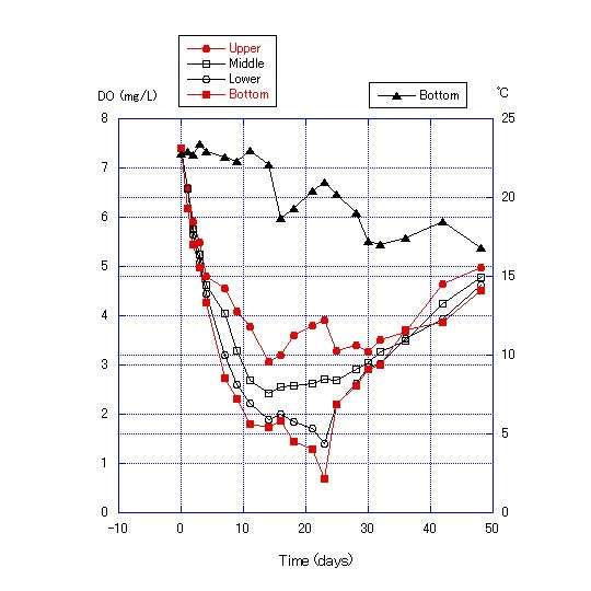 | Figure 8. Transition of dissolved oxygen concentration and bottom temperature for a water depth of 180 cm with addition of 0.125 g of cellulose powder to the sand in the bottom soil of the column |
The chemical properties of the water obtained from Lake Biwa are shown in Table 2, and the results of Experiment 2 are shown in Figures 7, 8 and 9. DO became lower with the addition of more cellulose to the bottom sand. For the addition of 0.125 g cellulose to 200 g sand, DO was lowest after 12 to 24 d, reaching a minimum of 0.68 mg/L. After 23 d, DO values recovered (Figure 8). For the addition of 0.25 g of cellulose, DO became near zero after 12 d and anoxia continued for about 2 weeks (Figure 9).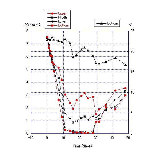 | Figure 9. Transition of dissolved oxygen concentration and bottom temperature for a water depth of 180 cm with addition of 0.25 g of cellulose powder to the sand in the bottom soil of the column |
The decrease of DO in the water column in Experiment 2 was due to the consumption of oxygen by microorganisms in the sand. Microorganisms consume oxygen in the decomposition of cellulose. Therefore, oxygen consumption is proportional to the cellulose content. Further, DO values were lower at the bottom layer for the first 12 to 28 d of the experiment, and differences in DO values among the four measurement points become greater day by day during this period, indicating that the rate of oxygen consumption by microorganisms out-paces oxygen diffusion from the upper to the lower layers. After days 24 to 30, the differences in DO values among layers become smaller and the values converge. This pattern indicates that the DO consumption by microorganisms either nearly stops or greatly diminishes. It is also expected that the oxygen diffusion from the upper layers becomes faster than DO consumption by microorganisms and that oxygen diffusion from the upper layers increases, such that the DO concentration in all four layers converges after about 30 d.The results of Experiment 3 are shown in Figures 10 and 11. The thermocline was formed by adding water warmed to 30C to the top of water at 24C. The thermocline was maintained in the water column through the use of an electric blanket during the experiment, and the temperature range of the lowest layer shifted only from 24 to 27C, and the uppermost layer only from 37 to 38C after 435 h.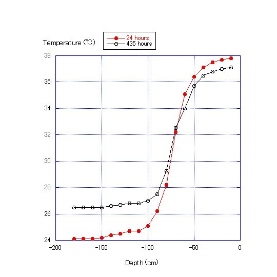 | Figure 10. Water column temperature at 10-cm intervals at 24 and 435 h |
Figure 11 shows that DO at the depth of 170 cm immediately increased from zero to 0.85 mg/L after 1 h and to 3 mg/L after 24 h. Water in the upper layer was at a higher temperature and did not mix easily with water of lower temperature in the lower layer due to the difference in density. The oxygen supplied to the lower layer was considered to not be a result of mixing the upper and lower layers but rather through diffusion from the upper layer, as reflected in the immediate decrease in DO at depths of 60 and 20 cm. Rapid changes in DO in the column layers continued only for about 24 h and after that, stabilized or only decreased slightly over time.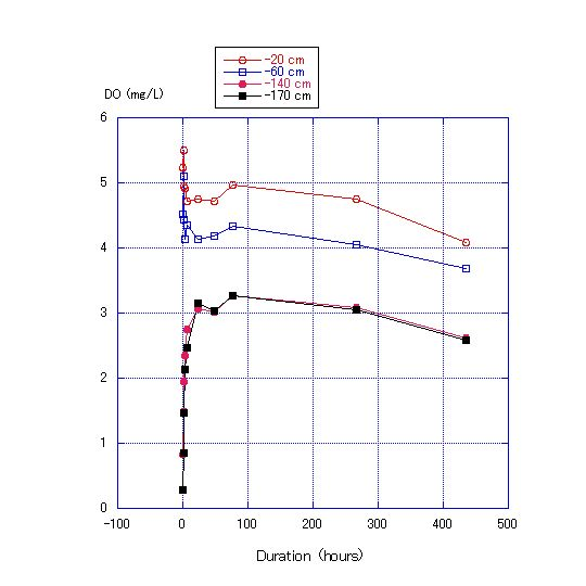 | Figure 11. Transition of DO concentration at depths of 170, 140, 60, and 20 cm in the column used in Experiment 3 |
There was no difference in the DO between depths of 140 and 170 cm (Fig. 11), but there were differences in DO between depths of 60 and 20 cm. After 435 h, the temperature was almost constant (26.5C) at the depths of 140 to 170 cm, but showed a range of 34.0 to 37.0C at 60 to 20 cm. In this experiment, the thermocline was formed between depths of zero to 100 cm. Formation of the thermocline prevents the vertical diffusion of DO. Thus, differences in DO would not disappear until the differences in temperature dissipate.Formation of a thermocline in the water column makes it difficult for the layers to mix and may lead to a difference in DO. Further, the results of Experiment 3 show that prevention of diffusion also leads to differences in DO between water layers.The low DO concentration in the seawater body affects fish because generally fish need the high DO concentration to live in it and from Equation (4) showing that DO is more likely to increase in shallow water along natural shorelines than in deep water near constructed seawalls, fish are expected to be more active along natural shoreline areas. Further, from Experiment 2, sea sediment in coastal areas with vertical seawalls with the same amount of organic matter as in a shallow water area will more easily develop hypoxia and anoxia (Figure 12).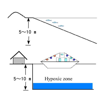 | Figure 12. Comparison of two types of shorelines. Shorelines with beaches tend to have seawater that is rich in DO and where fish are active. Shorelines with vertical seawalls tend to develop areas of hypoxia |
In Japan, there were many beaches along the coasts of Tokyo Bay, Ise Bay and Osaka Bay. However, land reclamation efforts and development of seaports starting decades ago has led to the construction of vertical seawalls along the shorelines. It is expected that the quality of the inshore fishery in these bays became low from this point.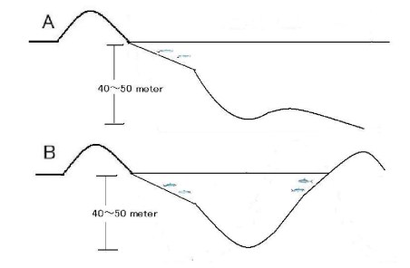 | Figure 13. Comparison of the topography of two types of shorelines: A shoreline with a steep drop-off and B shoreline with islands nearby |
Figure 13 shows the topography of bays with nearby islands. The sloping topography makes it more likely that DO will be sufficient to support an inshore fishery. In Japan, the Seto Inland Sea area, which has many islands, shows this topography.From the results of Experiments 1 and 2, it is thought that there are several layers of differing DO concentrations in ponds and lakes (Figure 14). From the results of Experiment 3, it is considered that when a thermocline is present, the differences of the DO concentrations between the layers will become larger.In many areas of the world, hypoxia is reported with the presence of thermoclines and haloclines. These phenomena are related by three factors: diffusion of oxygen in water, consumption of oxygen by microorganisms and development of pycnoclines.Burns[5] showed that a thermocline was developed in the central basin of Lake Erie, resulting in a difference in oxygen saturation percentage between the hypolimnion and the epilimnion. Further, the increased temperature in the bottom water from August to September coincided with a period of anoxia from September 23-27. Our results from Experiments 2 and 3 show that microorganism activity in the bottom sediment and establishment of a thermocline induce hypoxia.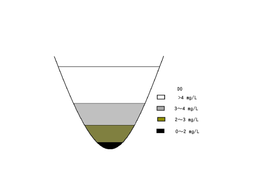 | Figure 14. The formation of stratification and water layers with different DO concentrations in ponds or bays |
Hawley et al.[6] reported an area of hypoxia in the hypolimnion of Lake Erie in September 2005. The area of oxygen concentration under 4 mg/L coincided with depths of 20 m or greater in the central basin of Lake Erie[6]. These phenomena can be explained by the findings demonstrated in Experiments 1, 2 and 3. In contrast, DO was higher in the eastern basin than in the central basin, despite that the eastern basin is deeper. This summer phenomenon is thought to be influenced by the lower temperature and consequently lower microorganism activity of the bottom layer in the eastern basin[5].Figure 15 shows the relationship between DO, salinity, and temperatures in Tokyo Bay. The halocline was first formed on July 19, 2010, but from July 19 to July 20, there was no thermocline until July 21 when the temperature of the bottom layer became lower than before and hypoxia developed. This phenomenon can be explained by an intrusion of fresh seawater from other places near the monitoring point. In this case, hypoxia developed even with a decrease in bottom temperature, which is expected to dampen bacterial activity, due to the formation of a themocline and halocline.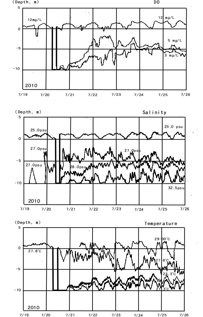 | Figure 15. Mid-summer DO, salinity, and temperature profiles at the Tokyo Monitoring Post in Tokyo Bay |
In Tokyo Bay, according to data from August 3 to August 8 in 2010, differences in DO between water layers often almost disappears in short (1-d) periods when there is a turnover of the water column. Following these events, DO increases, as mixing is a much more efficient mechanism for delivering DO to the bottom layers than is diffusion through the water column.Conley et al.[7] reported the depth and spatial distributions of hypoxia in the Baltic Sea using data from the Baltic Environment Database at Stockholm University. When these two data sets in the report are compared, it is supposed that the spatial distribution of hypoxia in the Baltic Sea corresponds to the depths greater than 100 m.In the Baltic Sea, the influence of the halocline must also be considered. However, since both of the halocline and the thermocline are pycnoclines, the effect of the halocline is expected to foster differences in DO in the seawater layers based on the results of the Experiment 3.The Baltic Sea is a semi-enclosed sea and is not expected to be influenced by ocean currents. Therefore, it is expected that seawater layers developed through the formation of a pycnocline are not disturbed by ocean currents and may be persistent, leading to the maintenance of hypoxia over extended periods.Costantini et al.[8] reported the effect of hypoxia on habitat quality for striped bass in Chesapeake Bay and showed that the development of a thermocline in Chesapeake Bay corresponded well with the DO profile[8]. Sanford et al.[9] showed the correlation between the development of the halocline in Chesapeake Bay and the DO profile, but the degree of correspondence was less than for the thermocline. This phenomenon is similar to the results from the Tokyo Monitoring Post where hypoxia was first induced by the presence of the thermocline because a thermocline is more effective than a halocline for inducing hypoxia.Wei[10] reported that hypoxia formed in areas adjacent to the Changjiang Estuary and that both a thermocline and halocline were present. Other factors, such as tidal currents and the distribution of Chl-a and turbidity in the estuary were also investigated, and the hypoxia zone were reported. In the Changjiang Estuary, it is expected that all three of these factors (oxygen diffusion, pycnocline development and oxygen consumption) are inducing hypoxia occurred in this area.The formation of a halocline at the surface to depths of 100 m in the southern Black Sea closely corresponding to DO and salinity profiles was reported by Basturk et al.[11]. These findings from the field support the results obtained from Experiment 3 showing that a pycnocline inhibits oxygen diffusion from the air such that the DO concentration in seawater deeper than 100 m becomes zero due to the presence of the pycnocline.Further, hydrogen sulfide is present in the southern Black Sea at depths deeper than 100 m[11], showing that seawater at these depths is in a reducing state. Since the Black Sea is an enclosed sea, there is no mixing of seawater layers by ocean currents. Therefore, oxygen is only supplied to the southern Black Sea through diffusion from the air and through limited inflowing river water. Therefore, diffusion from the air is the major source of oxygen supply, and it only reaches to depths of 100 m. For these reasons, the Black Sea would be in a reducing state at depths deeper than 100 m and permit sulfate reducing bacterium to proliferate in the sea sediment.
4. Conclusions
One equation was obtained to describe the recovery of DO concentration in a water column. There are three factors that determine the DO concentration in a water column with the soil at the bottom in order from slow to fast: rate of diffusion of oxygen across the air-water interface, diffusion within the water column, and rate of oxygen consumption by the sediment microorganisms The formation of a thermocline prevents oxygen from diffusing within the water column and induces differential DO concentrations across layers.The findings in these laboratory experimental set-ups corroborate observations in natural water bodies. For example, beaches of coasts and bays with islands are more favorable for fish and shellfish and bottom layers of ponds with organic sediments easily become hypoxic and/or anoxic. Hypoxia and anoxia are observed worldwide in water bodies such as Lake Erie, Chesapeake Bay, Baltic Sea, Tokyo Bay, Black Sea and the Changjiang Estuary. The phenomena of hypoxia and/or anoxia developing in these areas can be explained by the mechanisms partly demonstrated in these laboratory experiments.Considering the results obtained above, it is important to determine the accurate three rates concerning dissolved oxygen concentrations. By determining these rates, it is supposed that we will be able to know when and where hypoxia and anoxia will be induced in these sea areas.
ACKNOWLEDGEMENTS
We thank the Japan Coast Guard for making various data on Tokyo Bay available on the Internet through their management of the Tokyo Monitoring Post, and we thank Yasuhiro Senda and Maki Takada, students of the University of Shiga Prefecture, for assisting with the experiments.
References
| [1] | G. A. Truesdale, A. L. Downing, and G. F. Lowden, 1955, The solubility of oxygen in pure water and sea-water. J. Appl. Chem., 5, 53-62. |
| [2] | Sewerage Bureau of Tokyo Metropolitan Government. http://www.gesui.metro.tokyo.jp/kanko/kankou/17s_of_tokyo/06.htm, October 1, 2012. |
| [3] | Government of Aichi Prefecture.http://www.pref.aichi.jp/0000035313.html |
| [4] | Japan Coast Guard.http://www4.kaiho.mlit.go.jp/kaihoweb/index.jsp |
| [5] | N. M. Burns, 1976, Temperature, oxygen, and nutrient distribution patterns in Lake Erie, 1970. J. Fish. Res. Board Can., 33, 485-511. |
| [6] | N. Hawley, T. H. Johengen, Y. R. Rao, S. A. Ruberg, D. Beletsky, S.A. Ludsin, B. J. Eadie, D. J. Schwab, T. E. Croley, and S. B. Brandt, 2006, Lake Erie hypoxia prompts Canada-U.S. study, Eos, 87(32), 313-319. |
| [7] | D. J. Conley, C. Humborg, L. Rahm, O. P. Savchuk and F. Wulff, 2002, Hypoxia in the Baltic Sea and basin-scale changes in phosphorus biogeochemistry, Environ. Sci. Technol., 36, 5315-5320. |
| [8] | M. Costantini, S. A. Ludsin, D. M. Mason, X. Zhang, W. C. Boicourt, and S. B. Brandt, 2008, Effect of hypoxia on habitat quality of striped bass (Morone saxatilis) in Chesapeake Bay, Can. J. Fish. Aquat. Sci., 65, 989-1002. |
| [9] | L. P. Sanford, K. G. Sellner, and D. L. Breitburg, 1990, Covariability of dissolved oxygen with physical processes in the summertime Chesapeake Bay, J. Mar. Res., 48, 567-590. |
| [10] | H. Wei, Y. He, Q. Li, Z. Liu, and H. Wang, 2007, Summer hypoxia adjacent to the Changjiang Estuary, J. Mar. Systems, 67, 292-303. |
| [11] | S. T. Besiktepe, Ü. Ünlüata, and A. S. Bologa (ed.), 1999, Environmental degradation of the Black Sea: Challenges and remedies, Klumer Academic Publishers, 43-59. |
 Abstract
 Reference
 Full-Text PDF
 Full-text HTML