1. Introduction

Current methods of mechanical control have a robust heritage that hails from at least 1830 with Chasle’s theorems of motion Phoronomics [1], flowering in the last centuries [2-24] with both non-technical and technical aspects developed [25-66]. Contexts from the last centuries are renewed in this century, as nations threaten each other on a globe with multiple nations in space and the accompanying ability to strike each other with destructive weapon systems. Artificial intelligence is blossoming as the nations’ disparate government seeks competitive advantages for their national power. Despite the impetus in national security, artificial intelligence applied to economics has also been driven by the pursuit of wealth [52-53]. Advanced algorithms [31-62] for nonlinear adaptive system identification [48-53] and control [42-50] permitting improved performance of space missions [31-33, 55] arise in a time when the United States has discovered a pre-occupation with low-end conflicts in the middle east amidst an increasing belligerent world of threats [29-33]. This realization culminated in the recent edict to create a new military service in the U.S. purely dedicated to space [61].

The manuscript emphasizes feedforward controllers, trajectory tracking, and automatic trajectory generation, highlighting a key feature of deterministic artificial intelligence requires autonomous trajectory generation. This article discusses recent research in the underlying technologies of deterministic (non-stochastic) artificial intelligence applied to spacecraft.

1.1. Rotational Mechanics…also known as “the Dynamics”

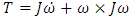
As described by Kane [18] Spacecraft rotate in accordance with rotations in accordance with Euler’s Moment Equations [3], where m is the mass of the object and [J] is a matrix of mass moments of inertia; meanwhile kinematics [6] are mutually equivalent expressions of the inertial values in Euler’s equations. “The dynamics” are comprised of the kinetics described in Euler’s equations together with a chosen set of kinematics [60].

1.2. Kinematics

Several options are available to describe the inertial components of Euler’s equations, and researchers may choose kinematics to maximize their convenience and priorities. Reference [60] critically investigates kinematics expressions, revealing strengths and weakness of various forms. Key parameters used in the critical analysis include speed-of-computation and accuracy of representations providing a menu of options from which researchers can choose.

1.3. Trajectory Generation

The aforementioned feedforward architectures rely on modeling of dynamic system equations, and furthermore the control equations will be seen to necessitate formulation of a desired full-state trajectory: at least angular velocity and angular acceleration trajectories to formulate the control in addition to angular position to formulate the error. A key feature of deterministic artificial intelligence is the necessity of autonomous trajectory generation, and this feature is a main focus of this manuscript.

2. Materials and Methods

2.1. Rotational Mechanics Fed by Autonomous Trajectory Generators

Figure 1 displays the topology of this investigation. Step inputs are accepted from users despite its mathematically singular form. These inputs demand the immediate task of autonomous trajectory generation to create mathematically smooth angular velocity and acceleration inputs for the control calculation. This calculation is performed by he deterministic artificial intelligence engine residing in the block labeled Actuators and Control. The control toques together with external disturbance torques are fed to Euler’s equations of motion contained in the block labeled System Dynamics.

Figure 1. System topology with artificial intelligent elements (equations 5,6,7) in the Actuators & Controls block requiring autonomous trajectories (per equations 9,10,11) to command the System Dynamics (per equations 1-4) in the face of arbitrary, unknown External Disturbances

2.1.1. Necessity for Smooth Trajectories

Cooper and Heidlauf [48] elaborate the issue of non-smooth trajectories with the following short illustrative expansion. Figure 2 illustrate three options for (one) smooth trajectory and (two) non-smooth trajectories.

Figure 2. Desired angle, rate, and acceleration trajectories evaluated for thirty seconds (abscissa)

Reference [48] reveals that any non-smooth feature in the commanded trajectory represents an unrealistic demand of a physical system and such should be avoided. Non-smooth points induce dramatic, unstructured excitation to the learning algorithm that carries only deleterious effects.

2.2. Dynamics

The physics-based dynamics are the foundation of deterministic self-awareness. Referring back to Figure 1, the Dynamics block contains equation 2 and a torque is provided by the Feed Forward Control section fed by the Torque Generator (the far left inputs of the topology). Equation (2) is equivalent to equation (1) expressed in body coordinates. 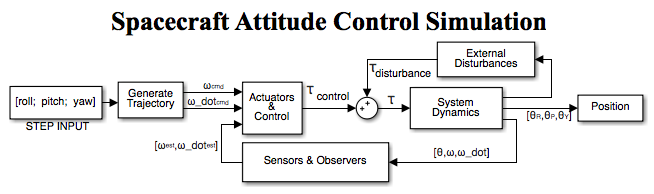In equation (1), m is the mass of the object and [J] is a matrix of mass moments of inertia; while denotes the time-derivative, .

(1)

(2)

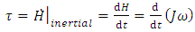
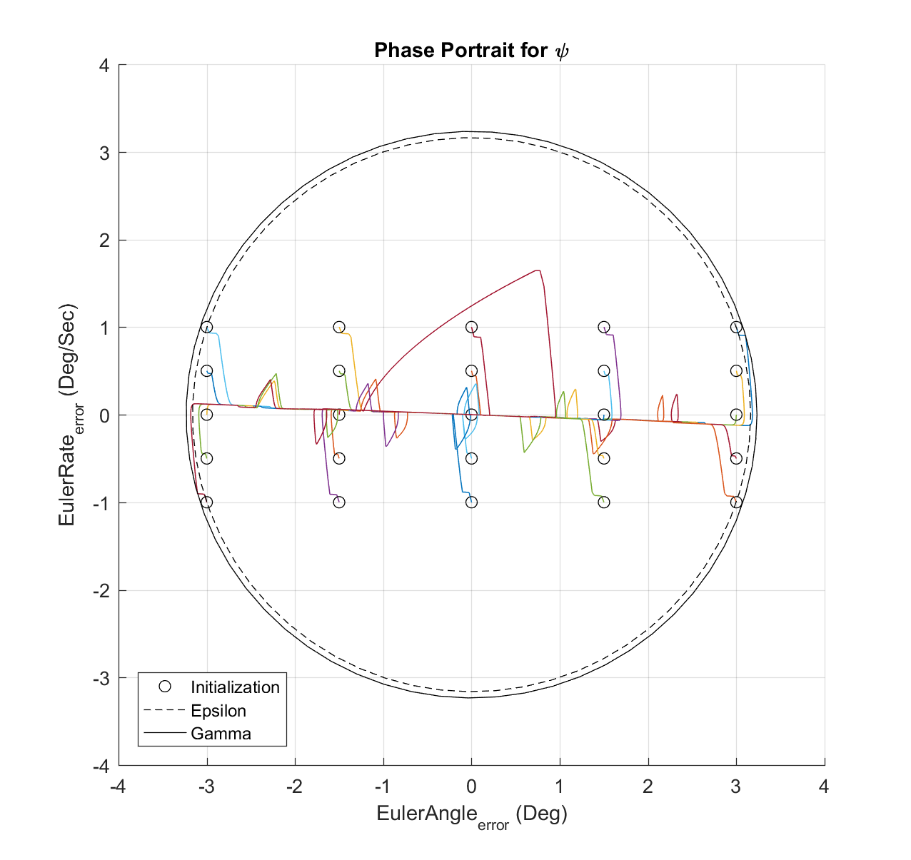
Equations (1) and (2) are versions of the governing dynamics where J is a matrix containing mass moments of inertia, angular velocity is depicted as , while angular acceleration is depicted by . Coupled motion in the governing equations of dynamics are evident in the term of equation (5), where is the angular momentum whose time-rate of change is . Motion is all axes results from any motion in any axis due to the coupling terms, and the amount of motion in each axis is scaled by the mass moment of inertia terms, which behave like “gains”.

Manipulation of equation (2) help isolate the angular velocity of the body per [60]. Differentiating yields the angular acceleration which appears in the produt , permitting multiplication by the matrix inverse [J]^-1 and then integrated as per equations 2 and 3. Kinematic Euler Angles are calculated from these angular velocity displayed in equation (3).

(3)

(4)

Equation (4) illustrates how the dynamics in equation (2) form the basis of self-awareness. Notice the two equations are equivalent except equation (4) is designated as the desired torque command with subscript letter d. This equivalence acknowledges the dynamics as a statement of self-awareness, and therefore is the exact structure of the deterministic artificial intelligence control command. This command provides the structure for learning, and several instantiations of learning are explored in section 2.3, where the input to the learning algorithms is trajectory tracking errors.

2.3. Determinisitic Artificial Intelligence

The Actuators and Control block of the topology in figure 1 contains the heart of the deterministic artificial intelligence algorithm, the ideal feedforward control that is formulated using the known-structure of the dynamics process governed by the inertial laws of rotational mechanics (i.e. Euler’s moment equations) in equations 1-4. The inside of the block is displayed for various parameterization of the deterministic artificial intelligence algorithm in figures 3-5 corresponding to equations 5-7. Equations 6 and 7 use a standard regression formulation of equation 4 to parameterize the problem permitting least squares learning algorithms in equations 6 and 7 respectively, where equation 4 is the first estimate, while equation 5 is the estimate correction. 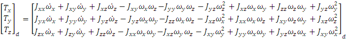in equations (4)-(6) include the regression parameterization of the feedforward control, where is a vector of mass moment of inertia components.

Figure 3. Feedforward in the Actuators & Controls block of Figure 1 parameterized by the learning-dynamics adapted by proportional-derivative feedback as defined in equation (5)

(5)

Figure 4. Feedforward in the Actuators & Controls block of Figure 1 parameterized by the learning-dynamics adapted by recursive least squares feedback as defined in equation (6)

(6)

Figure 5. Feedforward parameterized by the learning-dynamics adapted by extended least squares feedback as defined in equation (7)

(7)

Notice, as illustrated in the system topology in figure 1, the deterministic artificial intelligence engines of figures 3-5 required autonomous trajectories. Section 2.1.1 illustrated the impacts of non-smooth trajectories, and the remainder of this research utilizes simple smooth sinusoidal deterministic structures for autonomous trajectory generation. The next section examines various methods to calculate the trajectory revealing a family of choices yielding various accuracies with accompanying computational burdens.

2.4. Sinusoidal Trajectories

Prior to this point, we assumed a single method of sinusoid generation (MATLAB’s since function). In this section, the governing equation of feedforward control will remain unchanged from the sections above, but we investigate the impact of four different sinusoid generation methods in the Generate Trajectory block of figure 1, namely:

Ÿ MATLAB’s Sine Function

Ÿ 4th Order Taylor Series Approximation

Ÿ Low Precision Approximation Algorithm

Ÿ High Precision Approximation Algorithm

The effects of varying time-steps and commanded maneuver-time in feedforward control (everything to the left of dynamics block in figure 1) are investigates, in particular emphasizing the numerical accuracy and impacts on computational time for various methods.

To accurately model spacecraft maneuvers a standard sine curve is used,

(8)

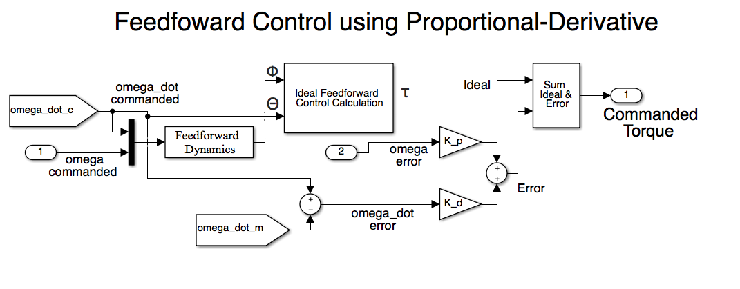
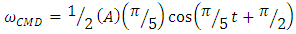
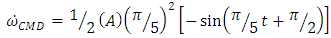
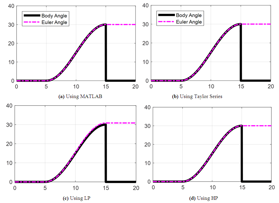
where A is the amplitude of the maneuver or the desired angular displacement of the spacecraft. The rate at which the spacecraft completes the maneuver is the frequency of the spacecraft denoted as . The phase on the sine curve, used to shift the trajectory curve for smooth onset, is denoted by . Using the Commanded Euler Angle and the Desired Slew time in conjunction with figure 1, the commanded maneuver is translated into a trajectory using various sine curves. Equation 8 above is elaborated with equations 9-11 below to investigate and compare numerical methods.

(9)

(10)

(11)

Using equation 9, the first and second time derivatives provide the commanded angular velocity and acceleration in equations 10 and 11. To ensure system stability, a quiescent time period is provided before the maneuver. The commanded trajectory is implemented over 5 seconds, after 5 seconds of quiescent time. The simulation is continued for 5 seconds after the commanded maneuver to provide sufficient settling time. The Actuator and Control Block in Figure 1 is fed by the trajectory generator and acts as the torque generator per equations 5, 6, and 7. The trajectory generator takes in a commanded body angle and then uses a sine wave in order to approximate the commanded maneuver. To help elaborate on this point, Figure 6 shows a square and a sine wave, both shifted up in amplitude such that they operate from zero to two instead of between negative and positive one.

Figure 6. Amplitude comparison of square wave to sine curve versus time in seconds

Figure 6 illustrates trajectory options: step function versus sinusoidal trajectory, as illustrated by a comparison of square wave to sine curve. The square wave illustrates expected behavior if a step function was used to approximate the commanded maneuver, the spacecraft would essentially be expected to transition from the zero position up to its max amplitude position instantaneously. This is a physical impossibility. With the sine wave in the same figure we can see that the spacecraft machinery is afforded a ramp up and slow down period along with a relatively linearly slope in the middle. Basically, the half period of sinusoid within the square pulse of Figure 6 is used to provide a smooth, achievable input to the system, where achievable in emphasized since step-inputs (or any other such discontinuous command) are not realizable by physical systems that lack an ability to instantly teleport from one location to another without any elapsed time.

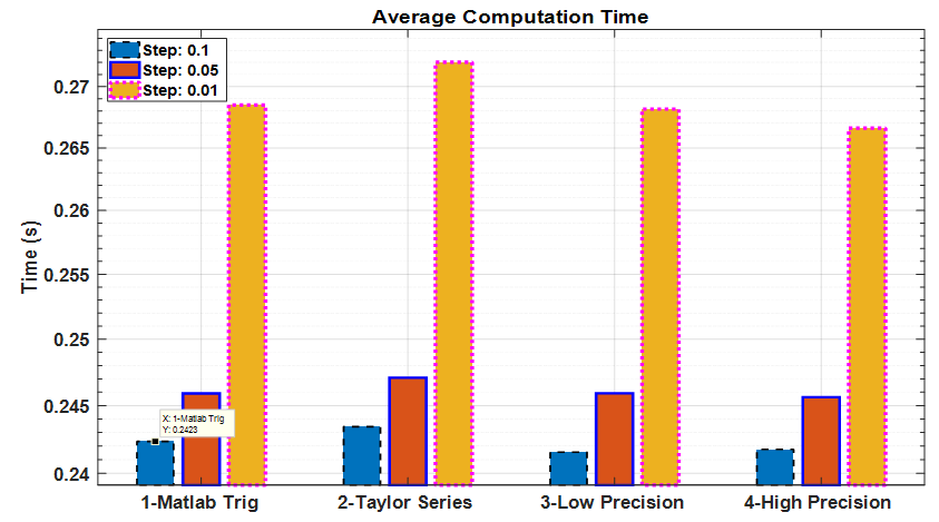
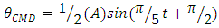
Our original model’s trajectory generator follows equations 12 through 14 to approximate the commanded maneuver for Angular Position, Angular Velocity (ω), and Angular Acceleration via the MATLAB sine wave function.

(12)

(13)

(14)

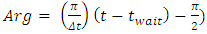
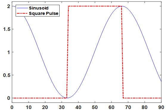
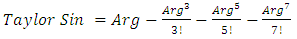
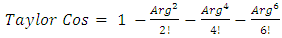
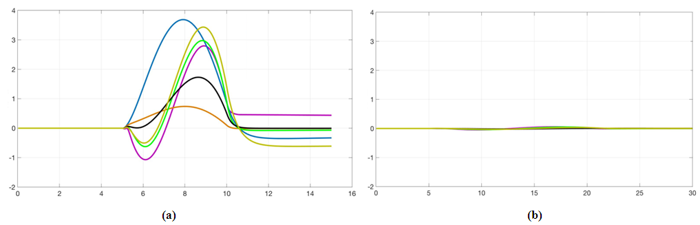
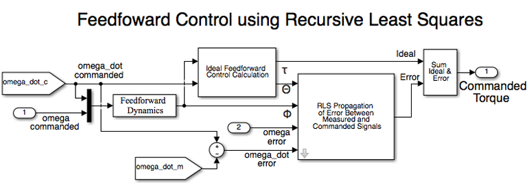
Equation 12-14 models the input command, where A is the maneuver’s commanded angle. The base frequency of the sinusoid is (π/Δt) where (Δt) is the desired maneuver time. The term allows for a quiescent period and -π/2 term allows for a proper phase shift to implement the sinusoidal half period of Figure 6. The effect of this can be seen later on in section 3. Equations 13 and 14 are just successive derivatives of equation 12 used to generate angular velocity and acceleration which are fed into the ideal feedforward control equations 5-7, which resides in the torque generator block of Figure 1. This produces an output torque which drives the Dynamics.

From equations 12-14 it can be clearly seen that the argument of the sine and cosine terms always follow the form of equation 15. We can use this to implement our Taylor Series and the other two other algorithms on equal footing.

(15)

The Taylor Series, as detailed in [62], is a numerical method that can be used to approximate other functions. In our model we substitute the sines and cosine from equations 12-14 with equations 16 and 17.

(16)

(17)

The Taylor Series is a power series and additional terms could be included ad infinitum for greater precision; however, initial testing found that 4 terms provided a reasonable approximation while maintaining a viable runtime. Additionally, it was found that pre-calculating the factorial terms sped up computation time.

The Low Precision (LP) and High Precision (HP) algorithms were found to be used in many applications, especially ones which required lower processing power such as mobile gaming. Ref [62] provided the baseline for adaptation of equations 18 and 19. Note that the same equation is used for sine and cosine expecting that the argument term is given a π/2 phase shift when applied to the cosine in equation 13. In equation 18, (+/-) indicates that a plus is used if Arg is less than zero and a minus is used otherwise.

(18)

(19)

Equation 319 provides additional smoothing to equation 15 at the cost of computation time to implement a high precision mode.

3. Results

This section describes the results of each of the major areas of investigation. Autonomous trajectory generation is used to evaluate computational efficiency and produce guidance to researchers about minimum step-size and numerical accuracy and computational time for several algorithms. Analysis is provided for comparison to the autonomous-rejection capability elaborated in the literature [42]-[57].

3.1. Continuous Versus Non-Continous Trajectories

The necessity for smooth trajectories claimed in section 2.1 is evaluated first by normalized comparison displayed in figure 2 with corresponding numerical results listed in Table 1.

Table 1. Comparison mean errors corresponding to figure 2

3.2. Stability Investigations

Stability of the combined system of deterministic artificial intelligence component algorithms is illustrated by nonlinear phase portraits in figure 8. The phase trajectories never exceed the arbitrary circle of non-infinite radius.

Figure 7. Yaw error (degrees) of iterated trajectories versus time in seconds with numerical assessment in table 1

Figure 8. Stability demonstration for Extended Least Squares Feedforward Controller, Traditional PID Feedback Controller, Enhanced Luenberger Observer, 15 Second Sinusoidal Trajectory

3.3. Trajectory Generation Computational Investigation

3.3.1. Solver/Integrator Step-Size

From a qualitative standpoint you can see that each sine generation algorithm created the intended Euler Angle movement shown earlier in Figure 6. Since we achieved the basic shape from each method (displayed in figure 9 where slight accuracy differences are visually apparent), we now turn our attention to analyzing the error and computation time associated with each for a given time step interval. We found that for a Runge-Kutta solver with step size of 0.01119, the MATLAB sine function “reached a point where CPU and MATLAB precision comes into play and shrinking step size does not necessarily result in reducing error”. With this in mind, step sizes of 0.1, 0.05, and 0.1 seconds were chosen for analysis, results of which can be seen in Figure 10 and Table 2.

Figure 9. 30° Yaw maneuver vs. time (seconds) with feedforward control for various methods

Figure 10. Computation Time Results

Table 2. Timing and Error Results

One major inference to be drawn from Table 2 is that the Normalized Error columns show Taylor, LP, and HP algorithms are roughly step-size invariant within our test range; only the MATLAB function’s error reduces with step size in our model. Interestingly, the LP and HP functions can be more accurate than Taylor but we are more concerned with the final angle in coarse control (corresponding to the peak of sine curve) rather than the intermediate steps – so in this case, the Taylor Series is considered more accurate.

The other major item of note is the difference in average computation time. While the MATLAB command is ultimately the most accurate at all step sizes, we can see that the LP and HP algorithms generally run faster. NOTE: Results were relatively inconsistent when run below 200 iterations but at 500 iterations we stabilized with HP and LP usually running faster during a given test. Since HP would run faster than LP sometimes and vice versa, even at greater iterations; it is believed that this may come down to specific CPU architecture used and how a dual core processor handles calculations.

4. Discussion

Regarding sinusoidal trajectory generation, if your design has accurate fine control (e.g., robust feedback mechanisms) and can handle coarse control error on the order of 10^-4, then it may be more prudent to utilize the HP algorithm, yielding reduced processing power and time resulting in lower power requirements and faster onboard calculations. A 4th order Taylor Series is not recommended, due to longer computation times and less accuracy than the MATLAB function; while extending the order of the series would increase accuracy but also extend its runtime, thereby, reducing viability. Additionally, simulation results reveal that the fastest methodology may vary with CPU architecture indicating that there may not be a definitive answer for “best” trajectory generation method. This should be evaluated within the specific spacecraft design trade space. Very little information is available on the proprietary MATLAB sine calculations but future testing will investigate the LP and HP algorithms against MATLAB on a variety of CPU architectures.

We developed a novel approach incorporating elements of deterministic artificial intelligence with extended least squares adapting an idealized feedforward controller compared to the standard recursive least squares optimal estimator realizing decreased mean error 23.4%, and standard deviation of the error 34.0%, while max error decreased 33.0%.

Future work should continue the line of research of Nakatani, Cooper, and Heidlauf, but implement their damage-tolerant feedforward methods and the latest developments in disturbance analysis [63] to fashion nonlinear feedforward autonomous disturbance-rejection controllers, taking advantage of the computational advice revealed in this study.

References

[1]  Chasles, M. (1830). "Note sur les propriétés générales du système de deux corps semblables entr'eux". Bulletin des Sciences Mathématiques, Astronomiques, Physiques et Chemiques (in French). 14: 321–326.
[2]  Merz, John (1903). A History of European Thought in the Nineteenth Century, Blackwood, London. p. 5.
[3]  Edmund Whittaker, A Treatise on the Analytical Dynamics of Particles and Rigid Bodies, Cambridge University Press, 1904, 1937.
[4]  Irving Porter Church Mechanics of Engineering, Wiley, New York, 1908; p. 111.
[5]  Thomas Wright, Elements of Mechanics Including Kinematics, Kinetics, and Statics, With Applications, Nostrand, New York, 1909.
[6]  Eduard Study (D.H. Delphenich translator), Foundations and goals of analytical kinematics. Sitzber. d. Berl. math. Ges. 1913, 13, 36-60. Available online at (accessed on 14 Apr 2017), http://neo-classical-physics.info/uploads/3/4/3/6/34363841/study-analytical_kinematics.pdf.
[7]  Gray, Andrew (1918), A Treatise on Gyrostatics and Rotational Motion, MacMillan, London, 1918 (published 2007 as ISBN 978-1-4212-5592-7).
[8]  Rose, M. E. (1957), Elementary Theory of Angular Momentum, New York, NY: John Wiley & Sons (published 1995), ISBN 978-0-486-68480-2.
[9]  Thomas Kane, Analytical Elements of Mechanics Volume 1, Academic Press, New York and London, 1959.
[10]  Thomas Kane, Analytical Elements of Mechanics Volume 2 Dynamics, Academic Press, New York and London, 1961.
[11]  William Thompson, Space Dynamics, Wiley and Sons, New York, 1961.
[12]  Donald Greenwood, Principles of Dynamics, Prentice-Hall, Englewood Cliffs, 1965 (reprinted in 1988 as 2nd ed.), ISBN: 9780137089741.
[13]  Ai Chzcn Fung and Benjumin G. Zimmermun (1969). Digital Simulation of Rotational Kinematics. NASA Technical Report NASA TN D-5302. October 1969. Washington, D.C. (https://ntrs.nasa.gov/archive/nasa/casi.ntrs.nasa.gov/19690029793.pdf).
[14]  D.M. Henderson (1977). Euler Angles, Quaternions, and Transformation Matrices – Working Relationships. McDonnell Douglas Technical Services Co. Inc., as NASA Technical Report NASA-TM-74839. July 1977. (https://ntrs.nasa.gov/archive/nasa/casi.ntrs.nasa.gov/19770024290.pdf).
[15]  D.M. Henderson (1977). Euler Angles, Quaternions, and Transformation Matrices – Working Relationships. McDonnell Douglas Technical Services Co. Inc., as NASA Technical Report NASA-TM-74839. July 1977. (https://ntrs.nasa.gov/archive/nasa/casi.ntrs.nasa.gov/19770024290.pdf).
[16]  D.M. Henderson (1977). Euler Angles, Quaternions, and Transformation Matrices for Space Shuttle Analysis. McDonnell Douglas Technical Services Co. Inc., Houston Astronautics Division as NASA Design Note 1.4-8-020, 9 June 1977. (https://ntrs.nasa.gov/archive/nasa/casi.ntrs.nasa.gov/19770019231.pdf).
[17]  Herbert Goldstein, Classical Mechanics 2nd Ed., Addison-Wesley, Massachusetts, 1981.
[18]  Thomas Kane, David Levinson, Dynamics: Theory and Application, McGraw-Hill, 1985.
[19]  Peter Huges, Spacecraft Attitude Dynamics, Wiley and Sons, New York, 1986.
[20]  William Wiesel, Spaceflight Dynamics, 2nd ed., Irwin McGraw-Hill, Boston, 1989, 1997.
[21]  Bong Wie, Space Vehicle Dynamics and Control, AIAA, Virginia, 1998.
[22]  Gregory G Slabaugh (1999). Computing Euler angles from a rotation matrix. 6(2000) 39-63. January 1999. (http://www.close-range.com/docspacecraftomputing_Euler_angles_from_a_rotation_matrix.pdf).
[23]  David Vallado, Fundamentals of Astrodynamics and Applications, 2nd ed., Microcosm Press, El Segundo, 2001.
[24]  Carlos Roithmayr, Dewey Hodges, Dynamics: Theory and Application of Kane’s Method, Cambridge, New York, 2016.
[25]  Timothy Sands, Richard Mihalik. Outcomes of the 2010 and 2015 nonproliferation treaty review conferences. World J. Soc. Sci. Humanities, 2: 46-51, 2016. DOI: 10.12691/wjssh-2-2-4.
[26]  Sands, T., 2016. Strategies for combating Islamic state. Soc. Sci., 5: 39-39. DOI: 10.3390/socsci5030039.
[27]  Mihalik, R., H. Camacho and T. Sands, 2017. Continuum of learning: Combining education, training and experiences. Education, 8: 9-13. DOI: 10.5923/j.edu.20180801.03.
[28]  Timothy Sands, Harold Camacho and Richard Mihalik, 2017. Education in nuclear deterrence and assurance. J. Def. Manag., 7: 166-166. DOI: 10.4172/2167-0374.1000166.
[29]  Timothy Sands, Richard Mihalik, (2018). Theoretical Context of the Nuclear Posture Review. Journal of Social Sciences, 14(1) 124-128, DOI 10.3844/jssp.2018.124.128. (http://thescipub.com/pdf/10.3844/jssp.2018.124.128).
[30]  Timothy Sands, Harold Camacho and Richard Mihalik, 2018. Nuclear Posture Review: Kahn Vs. Schelling…and Perry. Journal of Social Sciences 2018, Volume 14:145-154. DOI: 10.3844/jssp.2018.145.154.
[31]  Sands, T, 2009. Satellite electronic attack of enemy air defenses. Proc. IEEE CDC. 434-438. DOI: 10.1109/SECON.2009.5174119.
[32]  Timothy Sands, 2018. Space mission analysis and design for electromagnetic suppression of radar. Intl. J. Electromag. and Apps., 8: 1-25. DOI: 10.5923/j.ijea.20180801.01.
[33]  Timothy Sands, Danni Lu, Janhwa Chu, Baolin Cheng, Developments in Angular Momentum Exchange, International Journal of Aerospace Sciences, Vol. 6 No. 1, 2018, pp. 1-7. doi: 10.5923/j.aerospace.20180601.01.
[34]  Timothy Sands, Jae Kim, Brij Agrawal., 2006. 2H Singularity free momentum generation with non-redundant control moment gyroscopes. Proc. IEEE CDC. 1551-1556. DOI: 10.1109/CDC.2006.377310.
[35]  Timothy Sands, Fine Pointing of Military Spacecraft. Ph.D. Dissertation, Naval Postgraduate School, Monterey, CA, USA, 2007.
[36]  Jae Kim, Timothy Sands, Brij Agrawal, 2007. Acquisition, tracking, and pointing technology development for bifocal relay mirror spacecraft. Proc. SPIE, 6569. DOI: 10.1117/12.720694.
[37]  Timothy Sands, Jae Kim, Brij Agrawal, 2009. Control moment gyroscope singularity reduction via decoupled control. Proc. IEEE SEC. 1551-1556. DOI: 10.1109/SECON.2009.5174111.
[38]  Timothy Sands, Jae Kim, Brij Agrawal, 2012. Nonredundant single-gimbaled control moment gyroscopes. J. Guid. Dyn. Contr. 35: 578-587. DOI: 10.2514/1.53538.
[39]  Timothy Sands, Jae Kim, Brij Agrawal, 2016. Experiments in Control of Rotational Mechanics. Intl. J. Auto. Contr. Intel. Sys., 2: 9-22. ISSN: 2381-7534.
[40]  Brij Agrawal, Jae Kim, Timothy Sands, “Method and apparatus for singularity avoidance for control moment gyroscope (CMG) systems without using null motion”, U.S. Patent 9567112 B1, Feb 14, 2017.
[41]  Timothy Sands, Jae Kim, Brij Agrawal, 2018. Singularity Penetration with Unit Delay (SPUD). Mathematics, 6: 23-38. DOI: 10.3390/math6020023.
[42]  Timothy Sands, Robert Lorenz, “Physics-Based Automated Control of Spacecraft” Proceedings of the AIAA Space 2009 Conference and Exposition, Pasadena, CA, USA, 14–17 September 2009.
[43]  Timothy Sands, 2012. Physics-based control methods. Adv. Space. Sys. Orb. Det., InTech, London. DOI: 10.5772/2408.
[44]  Timothy Sands, “Improved Magnetic Levitation via Online Disturbance Decoupling”, Physics Journal, 1(3) 272-280, 2015.
[45]  Scott Nakatani, 2014. Simulation of spacecraft damage tolerance and adaptive controls, Proc. IEEE Aero., 1-16. DOI: 10.1109/AERO.2014.6836260.
[46]  Scott Nakatani, 2016. Autonomous damage recovery in space. Intl. J. Auto. Contr. Intell. Sys., 2(2): 22-36. ISSN Print: 2381-75.
[47]  Scott Nakatani, 2018. Battle-damage tolerant automatic controls. Elec. and Electr. Eng., 8: 10-23. DOI: 10.5923/j.eee.20180801.02.
[48]  Peter Heidlauf, Matthew Cooper, “Nonlinear Lyapunov Control Improved by an Extended Least Squares Adaptive Feed forward Controller and Enhanced Luenberger Observer”, In Proceedings of the International Conference and Exhibition on Mechanical & Aerospace Engineering, Las Vegas, NV, USA, 2–4 October 2017.
[49]  Matthew Cooper, Peter Heidlauf, Timothy Sands, 2017. Controlling Chaos—Forced van der Pol Equation. Mathematics, 5: 70-80. DOI: 10.3390/math5040070.
[50]  Timothy Sands, “Phase Lag Elimination At All Frequencies for Full State Estimation of Spacecraft Attitude”, Physics Journal, 3(1) 1-12, 2017.
[51]  Timothy Sands, 2017. Nonlinear-adaptive mathematical system identification. Computation. 5:47-59. DOI: 10.3390/computation5040047.
[52]  Sands, T., "The Catastrophe of Electric Vehicle Sales", Mathematics", 5(3), 46, 2017.
[53]  Sands, T., "Electric Vehicle Sales Catastrophe Averted by Deterministic Artificial Intelligence Methods", Applied Sciences, submitted to special issue Electric Vehicle Charging, 2018. ISSN 2076-3417.
[54]  Timothy Sands, Thomas Kenny, 2017. Experimental piezoelectric system identification, J. Mech. Eng. Auto, 7: 179-195. DOI: 10.5923/j.jmea.20170706.01.
[55]  Timothy Sands, 2017. Space systems identification algorithms. J. Space Expl. 6: 138-149. ISSN: 2319-9822.
[56]  Timothy Sands, “Experimental Sensor Characterization”, Journal of Space Exploration, 7(1) 140, 2018.
[57]  Timothy Sands, Armani, C., 2018. Analysis, correlation, and estimation for control of material properties. J. Mech. Eng. Auto. 8: 7-31, DOI: 10.5923/j.jmea.20180801.02.
[58]  “Remarks by President Trump at a Meeting with the National Space Council and Signing of Space Policy Directive-3”, Available online at the White House’s online news website: http://suo.im/4P2Duw (Accessed 20 June 2018).
[59]  Jack Kuipers, “Quaternions and Rotation Sequences, Geometry, Integrability, and Quantization”, Sept 1-10, 1999 Varna, Bulgaria; Coral Press, Sofia, 2000.
[60]  Brendon Smeresky, Alexa Rizzo, Timothy Sands, 2018. Kinematics in the Information Age. Mathematical Engineering, a special issue of Mathematics 6(9) 148. DOI: 10.3390/math6090148.
[61]  Kevin Bollino, Isaac Kaminer, Anthony Healey, Timothy Sands, 2018. Autonomous Minimum Safe Distance Maintenance from Submersed Obstacles in Ocean Currents. J. Mar. Sci. Eng. 6(3), 98.
[62]  Weisstein, Eric W. "Taylor Series. From MathWorld- A Wolfram Web Resource www.mathworld.wolfram.com/TaylorSeries.html.
[63]  Baczynski, Michael. Fast and Accurate Sine/Cosine Approximation, 18 July 2007, www.lab.polygonal.de/2007/07/18/fast-and-accurate-sinecosine-approximation/.
[64]  Keith Lobo, Jonathan Lang, Anthony Starks, Timothy Sands, 2018. Analysis of deterministic artificial intelligence for inertia modifications and orbital disturbances, International Journal of Control Science and Engineering, Vol. 8 No. 3, 2018, pp. 53-62. doi: 10.5923/j.control.20180803.01.
[65]  Timothy Sands, “Derivative Analysis of global average temperatures”, Climate, submitted to Volume (6), 2018.
[66]  Lucas Bittick, Timothy Sands, “Political Rhetoric or Policy Shift: A Contextual Analysis of the Pivot to Asia”, Journal of Social Sciences, submitted to Volume (14) 2018.