-
Paper Information
- Paper Submission
-
Journal Information
- About This Journal
- Editorial Board
- Current Issue
- Archive
- Author Guidelines
- Contact Us
Electrical and Electronic Engineering
p-ISSN: 2162-9455 e-ISSN: 2162-8459
2018; 8(1): 10-23
doi:10.5923/j.eee.20180801.02

Battle-damage Tolerant Automatic Controls
 Abstract
 Reference
 Full-Text PDF
 Full-text HTML
Scott Nakatani1, Timothy Sands2
1Space Systems Academic Group, Naval Postgraduate School, Monterey, USA
2Department of Mechanical Engineering, Stanford University, Stanford, USA
Correspondence to: Timothy Sands, Department of Mechanical Engineering, Stanford University, Stanford, USA.
| Email: |  |
Copyright © 2018 The Author(s). Published by Scientific & Academic Publishing.
This work is licensed under the Creative Commons Attribution International License (CC BY).
http://creativecommons.org/licenses/by/4.0/

The nature of adaptive controls, or controls for unpredictable systems, lends itself naturally to the concept of damage tolerant controls in high performing systems, such as aircraft and spacecraft. Recent technical demonstrations of damage tolerant aircraft prove the concept of adaptive controls in an operational environment. Research covered by this paper expands on the topic by discussing the application of adaptive controls to spacecraft and theory behind simulating damage tolerant control implementation. Simulation is then used to demonstrate the stability of adaptive controls when experiencing sudden mass loss and rapid changes in inertia.
Keywords: On-Orbit Damage, Autonomous Systems, Nonlinear Controls, Adaptive Controls, Luenberger, Modified PID Control
Cite this paper: Scott Nakatani, Timothy Sands, Battle-damage Tolerant Automatic Controls, Electrical and Electronic Engineering, Vol. 8 No. 1, 2018, pp. 10-23. doi: 10.5923/j.eee.20180801.02.
Article Outline
1. Introduction
- In the 1950s and 1960s, the North American X-15 rocket powered aircraft was pioneering the concepts and principles that would come to define modern powered flight. Among the ground breaking ideas proposed was a system of adaptive controls, or a controller that would take into consideration the changing operational environment to deliver appropriate control to the operator. Limitations of current technology abounded, leaving the X-15 with a successful, but severely limited adaptive control system. Since then, many limitations have fallen away, allowing for the first time employment of adaptive controls on a large scale, especially for space based systems.Space based operations pose significant operational and technical challenges. The job of maintaining orbit in the space environment is complex, yet operators must also contend with outside threats to their spacecraft. Threats to spacecraft include the space medium itself, conventional weapons, directed energy weapons, and electronic warfare. [1] One threat in particular is growing at an alarming rate; the threat of colliding with other orbiting objects. The advent of space use has introduced more than 39,000 traceable manmade objects into orbit, with over 16,000 large enough to be currently tracked. [2] Of these objects, approximately five percent are functional. [2] This leaves a vast majority of objects orbiting earth that have no means of maneuvering away from a collision.This population of orbiting objects, including spacecraft, rocket bodies, and debris is continuously growing. The risk of collision in space rises with the number of objects in orbit, and has the potential to create cascading, exponential increases in the number of objects orbiting earth. [3] This increase is best illustrated by the first ever accidental collision between two satellites, Iridium 33 and Cosmos 2251, which left distinct shells of debris across wide orbits. [4] This collision alone produced more than 2,000 traceable objects. [5]The situation is made worse by the actions of the international community. In 2007, China successfully tested a kinetic kill vehicle against a defunct weather satellite, Fengyun-1C, creating approximately 950 traceable objects and many smaller objects. [6] This debris is generally considered responsible for the sudden breakup of a Russian retroflection satellite in 2013, which was destroyed after passing through the debris cloud left by the Chinese test. [7] As the opportunity for collision increases due to advancing technology and increasing debris, protecting operational spacecraft must become a priority.Expanding reliance upon space assets and space based capabilities increases the opportunity for and consequences of a disruption. Weapon technology will continue to advance and spread. Orbital debris can take many years to deorbit and only seconds to create. These things will not change. Clearly satellites require greater levels of protection than ever before, and a promising technology may hold some answers for flight within and outside of the atmosphere.In 2008, the Rockwell Collins Company, sponsored by the Defense Advanced Research Projects Agency (DARPA) demonstrated damage tolerant controls (DTC) in an aircraft scale model, by jettisoning 60 percent of one wing and landing the model, all autonomously. [8] This research, driven largely by increased the United States reliance upon remotely piloted and autonomous aircraft, promises to increase survivability and counteract the input latency inherent to operating an unmanned aerial vehicle (UAV). DTC recovers operational control of a UAV before the operator knows it is damaged, making DTC a tremendous asset. Then, in 2010, Rockwell Collins and DARPA again demonstrated the ability to regain control of a damaged autonomous UAV, this time the operational RQ-7B Shadow, continue the mission, and land successfully. [9] All capabilities were performed via the remaining control surfaces only. This was accomplished using only autonomous software, with modifications called adaptive controls.Adaptive control is best defined as “…an approach to dealing with uncertain systems or time-varying systems.” [10] This infers the use of what is known as an adaptive controller, defined as “…a controller with adjustable parameters and a mechanism for adjusting the parameters.” [11] By these definitions, adaptive control is a specific kind of learning system that is generally considered appropriate when a system exhibits time variable dynamics. [12] The demonstration of DTC by the RQ-7B is enabled via the use of adaptive control through an adaptive controller.Concurrently, with the successes of Rockwell Collins and DARPA, researchers at the University of Illinois successfully modified the programming for a UAV using adaptive controls. [13] Using this modification the UAV was able to search for, and follow a moving ground based target autonomously. These demonstrations represent industry firsts and a tremendous step forward in the use of adaptive controls.The successful tests by the University of Illinois, Rockwell Collins, and DARPA with autonomous flight and adaptive controls have certain industry parallels. Machine learning has developed many optimized adaptive controls, such as the relatively new reward-weighted regression model. [14] This model was developed specifically to minimize the processing power required, possibly allowing for greater adoption of autonomous machine learning. Adaptive controls have also been designed to adjust for a rapidly shifting center of gravity on light cargo trucks by the Robert Bosch Company, dramatically increasing stability and reducing rollover risk. [15] Additionally, adaptive controls are making their way into consumer products in the form of vehicular adaptive cruise control. [16] Adaptive cruise control is performed via the controller maintaining the user set speed of travel and changing to match the speed of slower moving vehicles when encountered. [17] All of these examples utilize adaptive controls to compensate for rapidly changing systems. Industry success and product availability lends plausibility to the attempt to utilize adaptive controls for space based operations. The advantages of adaptive controls for spacecraft are seemingly boundless. In a study by the University of Florida, adaptive controls are shown to overcome the real world variations in torque seen when spacecraft utilize Control Movement Gyroscope (CMG) gimbals. [18] These variations in torque can make spacecraft attitude control all but impossible, especially for small satellites. Another application is the proposed space tug, which moves between defunct orbiting objects, collects them, and deorbits them. [19] Adaptive controls would enable the tug to compensate for unknown debris mass and maximize its fuel capabilities.As the space medium becomes more crowded across all orbits, the development of DTC for spacecraft will become a necessity. Adaptive autonomous operations have been called for in order to improve spacecraft survivability. [1] Threats to spacecraft exist at every period of their lifetime; from launch to operations and disposal. DTC and the recent developmental leaps in implementing adaptive controls present a possible answer to these evolving threats. This paper will discuss the history, problems associated with, and a simulated solution for providing damage tolerance via adaptive controls.The purpose of this research is to simulate a satellite with sudden mass loss and simulate adaptive controls to counteract the loss. DTC would be able to react to the loss much quicker than any human operator, giving the satellite the best opportunity to recover from damage. The question this research seeks to answer is: Are DTC possible for satellites in orbit?The methodology of this research begins with a literature review of the development of adaptive controls. Following that is a detailed description of the development of the satellite simulation. Last is the data collection and analysis of results.
2. Materials and Methods
- In the 1950s and 1960s, the National Aeronautics and Space Administration (NASA), the United States Air Force (USAF), and the North American X-15 rocket powered aircraft were pioneering the concepts and principles that would come to define modern powered flight. Launched in flight from the wing of a B-52A aircraft, the X-15 would fire its rocket engine, achieve the mission’s required altitude, and glide to earth for landing. Among the ground breaking ideas proposed was a system of adaptive controls, or a controller that would take into consideration the changing operational environment to deliver appropriate control to the operator. [20] Primarily what the X-15 proved was the utility of something called Gain Scheduling.
2.1. Gain Scheduling
- Gain Scheduling is a method of adapting known linear control technique to meet the challenges required of a nonlinear system. [10] By selecting enough points across the changing system and designing linear controls for each portion of the operation, it becomes possible to achieve adaptive nonlinear control. The primary concern when using gain scheduling is the lack of stability that can occur if the system becomes over saturated or departs from the programmed model. In 1967, oversaturated controls of the X-15 that Major Mike Adams was piloting prevented him from regaining control of the aircraft after deviating from the mission trajectory. [21] Major Adams was killed in the resulting breakup, and the X-15 program lost its funding the next fiscal year. NASA reports the lessons from the X-15 were the basis of the flight control system for the Apollo Lunar Excursion Module, and heavily influenced the Space Shuttle program. [21]
2.2. Adaptive Control
- Concurrently to the X-15 project, adaptive controls were being proposed and put to the test in many other fields, such as spacecraft control and machine tooling. In partnership with the Bendix Corporation, the USAF experimented with utilizing adaptive controls with feedback for metal cutting, one of the first such attempts. [22] The goal was to account for tool wear in the machining process, both by measurement and by position feedback. At the same time NASA was investigating the possibility of developing adaptive controls for space vehicles, though the stated purpose was to extend the lifetime of spacecraft by minimizing the fuel consumption required to perform the mission. [23] Gain scheduling was heavily favored in these applications, as the required computing power to perform nonlinear adaptive control was yet to come. Gain scheduling requires significant up front processing power, in order to develop all the linear controls needed, which also suffered from the relative lack of computing power of the era.These projects led naturally to the inclusion of adaptive controls in the development of the International Space Station, to assist with stability during the construction phase and overall attitude control. [24] In this we see the emergence of developing inherently robust controls across the entire mission profile, where only the parameters change between the different phases. Also emerging at this point are many different attempts to limit uncertainty for space based systems, such as the use of Kalman filters, model reference controls, and linear quadratics. [25] Indeed, the realization that slight disturbances can lead to system failure has forced the development these inherently robust controls, and leads developers to calculate uncertainty and feed it into the control parameters adjustment during operations. [26] As late as 1983, the equations required to perform adaptive control for complex space structures were too complicated to be run in real time. [27]Development up to the 1990s left space operations needing a controller that functions well across a system with changing operational conditions. Serious study at this point focused on utilizing the dominant control method of industry, the proportional integral derivative (PID) controller, which was developed for naval autopilots. [28] The adaptive PID controller works for a wide array of processes without requiring significant characterization of the system, all while outperforming other control methods, such as the generalized predictive control system. [29] This is due in part to the flexibility of the controller, which is demonstrated in the adaptive control scheme used by this simulation. Due to the nature of the PID equation, developers can take specific portions of the controller and adapt them for a specific use, such as the Proportional Derivative controllers proposed for use in space manipulators. [30] PID and PID derivative adaptive controls show significant promise when applied to space based controls.
2.3. Simulation Methodology
- The purpose of the simulation is to answer our research question “Are accurate and stable DTC possible for satellites in orbit?” Simulating ground conditions allows for continuation and validation of any results in the laboratory. The satellite was modeled in SIMULINK and the satellite block diagram is as shown in Figure 1.
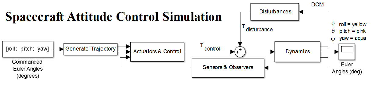 | Figure 1. Spacecraft Attitude Control Simulation |
2.3.1. Modified PID Controller
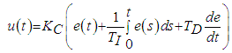
- The concept of the PID controller comes from the Åström and Wittenmark definition:
 | (1) |
 | Figure 2. Modified PID Controller |
2.3.2. Steering
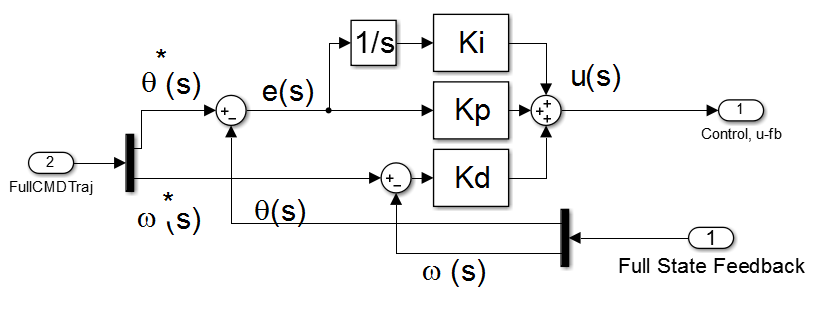
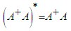
- The spacecraft achieves attitude control via CMG steering, within the CMG Steering subsystem, which is contained in the Actuators and Control subsystem as shown in Figure 1. The simulation uses a minimum, non-redundant CMG array of three CMGs and a balance mass to offset gravity gradient disturbances. The CMG Steering subsystem utilizes the Moore-Penrose Pseudoinverse Steering Law as described by Bong Wie. [31] Wie’s description assumes a CMG array as shown in Figure 3.
 | Figure 3. Steering Logic Pyramid Arrangement |
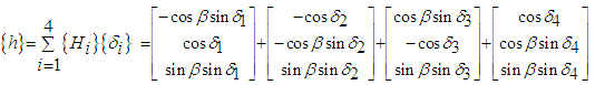 | (2) |
 is the pyramid skew angle, {Hi} is the angular momentum vector of the ith CMG, and
  is the gimbal angle of the ith CMG. Taking the time derivative of the angular momentum vector results in the equation:
 | (3) |
 is the gimbal angle vector, {ai} is the ith column of the Jacobian matrix [A] defined as:
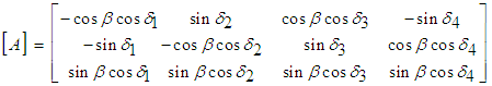 | (4) |
 , the CMG momentum rate command
  is defined as:
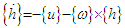 | (5) |
 is the angular velocity. Finally the Moore-Penrose Pseudoinverse Steering Law, also known as pseudoinverse steering logic, may be obtained as:
 | (6) |
 is the pseudoinverse of [A] if:
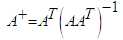 | (7) |
 | (8) |
 | (9) |
 | (10) |
 | (11) |
 , is the conjugate transpose of [A], a relationship otherwise known as Hermitian matrices. As the simulation uses only 3 CMGs, [A] in the simulation is a [3x3] square, real matrix. Therefore, the conjugate transpose of [A] is equal to the inverse of [A] and the pseudoinverse of [A]:
 | (12) |
 , to find the commanded gimbal rate, which is in turn sent to the gimbal actuators. Integrating the gimbal rate gives the gimbal state, which is an input of [A]. The subsystem outputs angular momentum rate or torque rate after multiplying [A] with the gimbal rate. The CMG Steering subsystem is as shown in Figure 4.
 | Figure 4. CMG Steering |
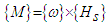
2.3.3. Dynamics
- The Dynamics section was derived from the law of conservation of angular momentum, and the definition of angular momentum:
 | (13) |
 the spacecraft angular velocity. From the definition of angular momentum comes Euler’s second law of motion:
 | (14) |
 | (15) |
 | (16) |
 | Figure 5. Spacecraft Dynamics |
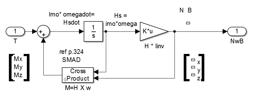
2.3.4. Kinematics
- The Kinematics section begins with the angular velocity components of the spacecraft,
 , and adds the angular velocity of the spacecraft’s orbit, resulting in
  , the angular velocity with respect to orbit. This angular velocity is transformed into a quaternion, which is a specific type of complex number, by the relationship:
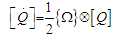 | (17) |
 is the quaternion,
  is the rate of change of the quaternion, and
  is the angular velocity with respect to orbit. Expanded, Equation 17 becomes the kinematic differential equation for quaternions in equation 19:
 | (18) |
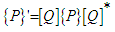 | (19) |
 | (20) |
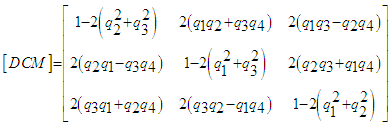 | (21) |
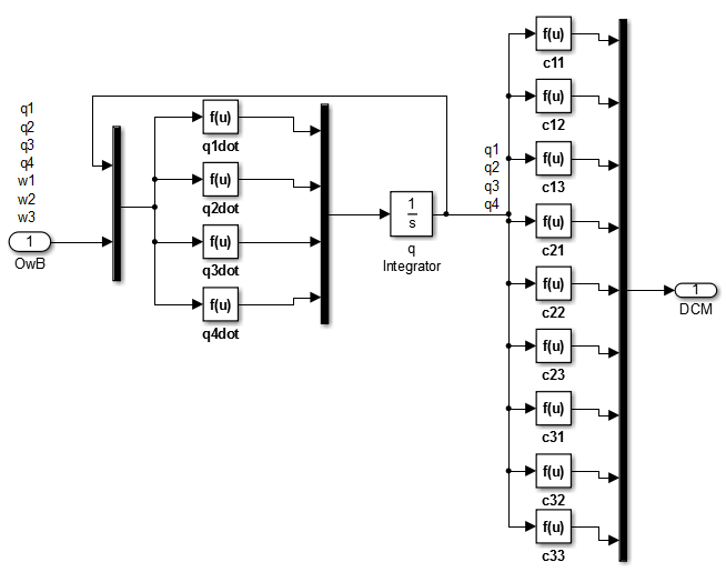 | Figure 6. Quaternion and DCM Calculation |
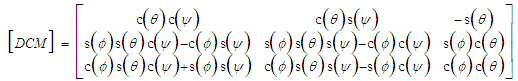 | (22) |
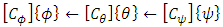 where
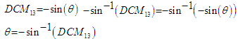
where  is the rotation matrix about the ith axis with an angle of x. [34].Having used Equation 21 to populate the DCM with values, the simulation uses Equation 22 to find the corresponding Euler angles. Pitch, or
  , can be found by taking the value of the first row, third column of the DCM, DCM13, applying the corresponding portion of Equation 22, and then isolating
  :
: | (23) |
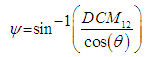
 found, the remainder of the Euler angles can be similarly isolated and solved:
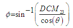 | (24) |
 | (25) |
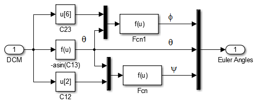 | Figure 7. Euler Angle Generator |
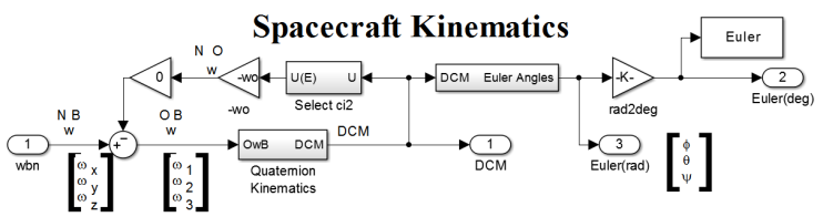 | Figure 8. Spacecraft Kinematics |
2.3.5. Disturbances
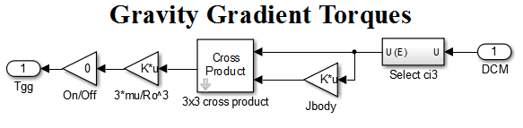
- The only disturbances modeled were the gravity gradient torque, or the torque due to unequal gravitational pull on the disparate parts of the satellite. This disturbance is expected to be observed in a laboratory follow up of this simulation. Gravity gradient torque is defined as:
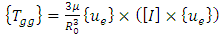 | (26) |
 is the Earth’s gravitational coefficient, R0 is the distance from Earth’s center, {ue} is the unit vector towards Nadir, and [I] is the spacecraft moment of inertia matrix. [32] The unit vector towards Nadir is picked out of the DCM:
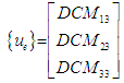 | (27) |
 | Figure 9. Gravity Gradient Torques |
2.3.6. Sensors and Observers
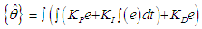
- The enabling concept behind the feedback capabilities of the simulation is contained in the Sensors and Observers block. Euler angles and angular rates enter, combined in a state vector, which can be shunted along different paths, from an unedited ideal full state feedback to sensor feedback, observers, state feedback, Kalman filtered sensors, and Lowpass filtered sensors. Once the simulation selects anything other than ideal full state feedback, a sensor is simulated. The sensor is the ideal feedback signal with a random number generator adding noise. Next in the process flow is the Observer Subsystem, containing a Luenberger observer and a PID observer. The purpose of any observer is to create a complete state vector from incomplete and/or noisy observations. The PID observer relies upon the same concept as the PID controller, or measuring current error, accumulating past error, and predicting future error. The PID observer equation, derived from Equation 1, is:
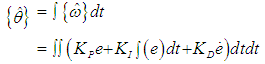 | (28) |
 is the estimated Euler angle,
  is the estimated angular velocity, e(t) is the error defined as e=uc-y where uc is the reference value, y(t) is the process output, and KP, KI, and KD are gain constants used to tune the observer. The PID controller operates by accepting angle data which is used to estimate the angular acceleration used to produce the angle data. Integrating this estimate gives estimated angular velocity
  , integrating again produces estimated Euler angles
  . Tuning the gain constants KP, KI, and KD such that the estimates approach the actual values, or
  and
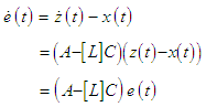
and  , achieves what is known as full state feedback.The other choice for observer, the Luenberger observer, also has the ability to receive the control signal from the Dynamics block, labeled TotalControl on the block diagram. The Luenberger observer operates on a system defined as:
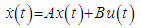 | (29) |
 | (30) |
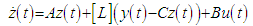 | (31) |
 | (32) |
 | (33) |
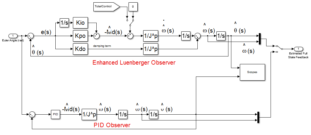 | Figure 10. Observer Subsystem |
 | (34) |
 is the state,
  is the transition matrix,
  is the control matrix,
  is the control, and
  is the process noise, all at time k. [37] The filter makes observations defined as:
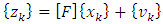 | (35) |
 is the observation,
  is the observation matrix, and
  is the observation noise. Both process and observation noise are assumed to normally distributed with covariance Q and R respectively. With these definitions, the Kalman filter makes estimates via this equation:
 | (36) |
 is the estimated state and
  is the Kalman gain. Using these relationships a Kalman filter makes a prediction of the state and covariance, calculates gain, and updates its state and covariance model. In the simulation, the state vector is broken apart, and the Euler angles are run separately from the angular velocity through corresponding Kalman filters. This enables the simulation to find the true error in the Kalman values by comparing the filtered Euler angles to be compared to the true Euler angles. The Kalman Filter block diagram is as shown in Figure 11.
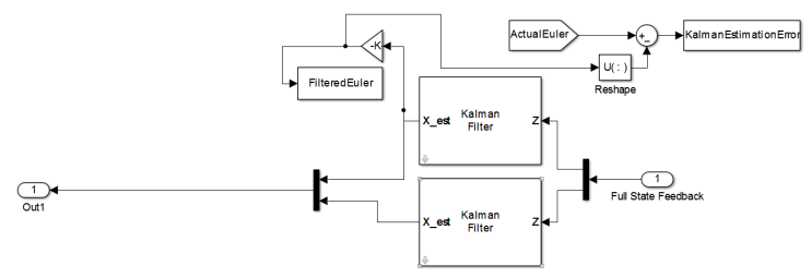 | Figure 11. Kalman Filter |
 | (37) |
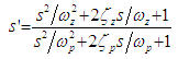
 are parameters tuned to the desired filter level [38] When the Lowpass filter is selected, the simulation breaks out each of the six components of the state vector, utilizes individual, separately tunable filters, and pushes the filtered signal to the Controller block. The Lowpass filter block diagram is as shown in Figure 12.
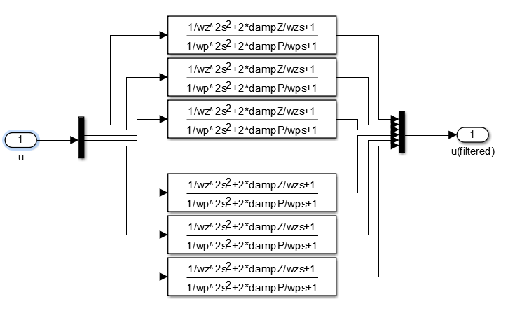 | Figure 12. Lowpass Filter |
 | Figure 13. Spacecraft Sensors and Observers |
3. Analysis and Results
- To answer the research question completely requires that the DTC are effective, accurate, and stable. This requires at least two different methods for analysis. The selected methods are the Monte Carlo analysis and phase portrait analysis. Both methods will demonstrate that DTC are effective, or that the simulated DTC do in fact function. The Monte Carlo analysis will also demonstrate the effects on accuracy due to DTC. The phase portrait analysis will demonstrate the stability of DTC.
3.1. Monte Carlo Analysis
- The Monte Carlo method, created by Stanislaw Ulam, draws its name from Ulam’s uncle, who frequented the Monte Carlo casino. [39] The premise is that by running simulations numerous times and recording the results, the outcome can be accurately characterized. This is akin to visiting a casino many times to determine the odds of any game of chance.In order to profile the outcome of the DTC in the simulation, a Matlab m-file was written, iteratively calling the simulation 900 times. Each iteration was distinguished by increasing the mass loss of the spacecraft by 0.1 percent, beginning at zero percent and finishing at 90 percent mass loss. Mass loss was simulated by reducing the simulated spacecraft moment of inertia matrix. This assumes that in the case of sudden mass loss, the satellite remains functional. Each iteration, the spacecraft was commanded to perform a 30 degree yaw, and the tracking error was recorded. In addition to the mean error, the standard deviation of the error was also recorded. The m file was written as shown in Appendix B.The Monte Carlo method applied to tracking error does an excellent job of characterizing the accuracy of the DTC when a spacecraft mass is suddenly lost, and by returning these results, shows that the DTC of the simulation do function correctly. The DTC never experienced greater than a mean 0.9 degree tracking error, with a standard deviation that was always less than 1.1 degrees. The results are as shown in Figure 14, where
 is the mean measured error, and
  is the standard deviation.
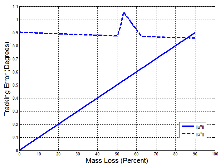 | Figure 14. Monte Carlo Analysis Results |
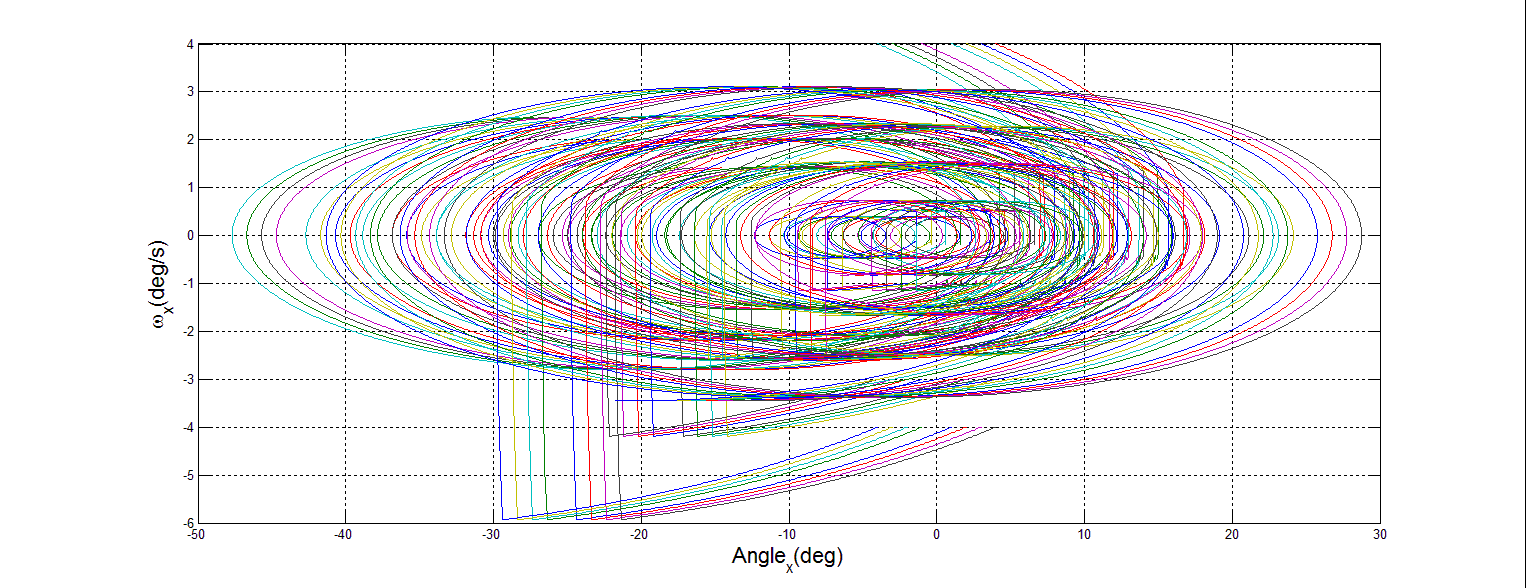
3.2. Phase Portrait Analysis
- The premise behind phase portrait analysis is to characterize the behavior of a system with regard to stability of equilibrium points. In this case, the behavior of the spacecraft DTC was examined around the commanded state vector. In order to demonstrate stability, the axes of angular rate and angular position in the inertial frame were chosen. If the motion described circles into the commanded point, then stability has been achieved.To create each phase portrait, a Matlab m-file was written which iteratively calls the simulation 36 times. Each portrait reflects fixed mass loss, with many different values of initial position and initial velocity. Mass loss was simulated by reducing the inertia matrix. This assumes that after sudden mass loss, the satellite remains functional. Each iteration changes the initial position and initial velocity, then records the results as the simulation is run for a set time of 100s. The omega value was already calculated by the Dynamics section, as variable w. In order to record the desired results, a new variable had to be captured, the position in the inertial frame. This was accomplished by adding an integrator block to the angular speed in the Dynamics section, and capturing the angle as the variable wAngles, as shown in Figure 15.
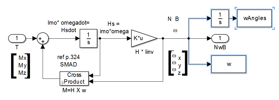 | Figure 15. Omega Angle Production |
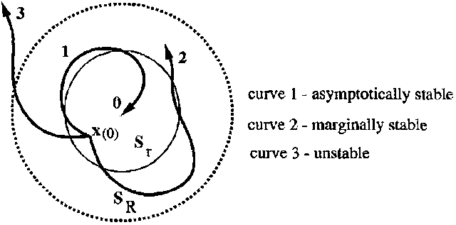 | Figure 16. Phase Portrait Stability |
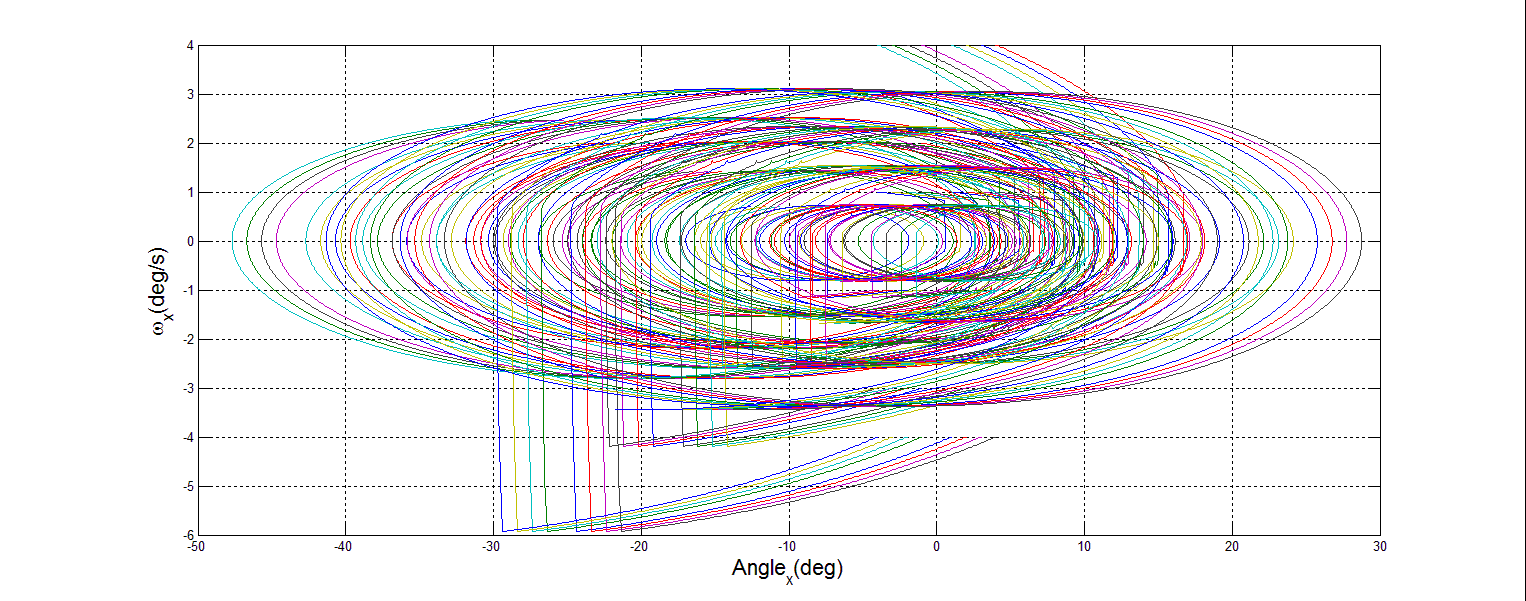 | Figure 17. 0% Mass Loss X Phase Portrait |
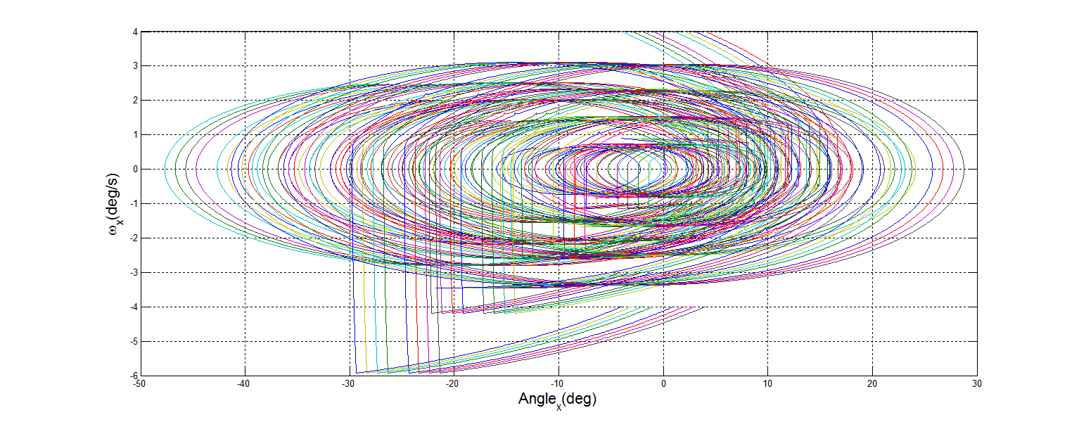
 | Figure 18. 45% Mass Loss X Phase Portrait |
 | Figure 19. 90% Mass Loss X Phase Portrait |
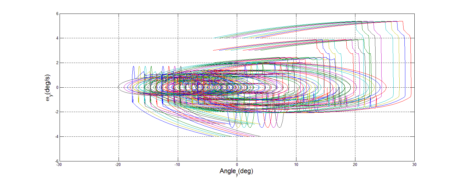 | Figure 20. 0% Mass Loss Y Phase Portrait |
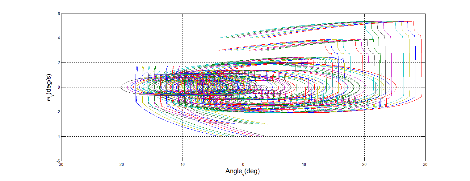 | Figure 21. 45% Mass Loss Y Phase Portrait |
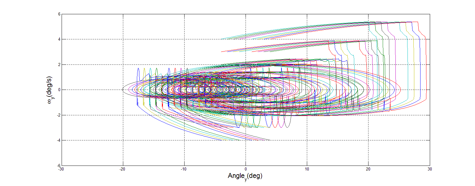 | Figure 22. 90% Mass Loss Y Phase Portrait |
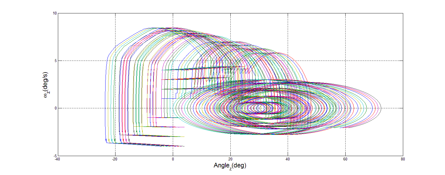 | Figure 23. 0% Mass Loss Z Phase Portrait |
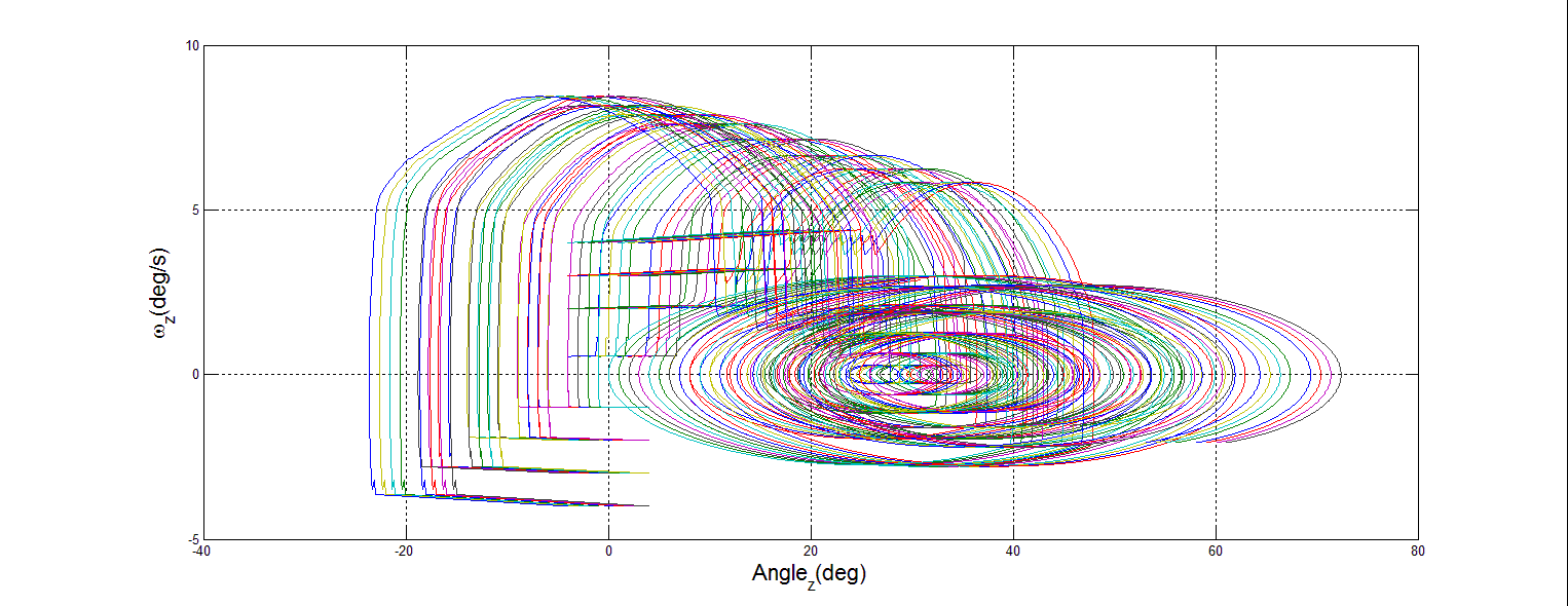 | Figure 24. 45% Mass Loss Z Phase Portrait |
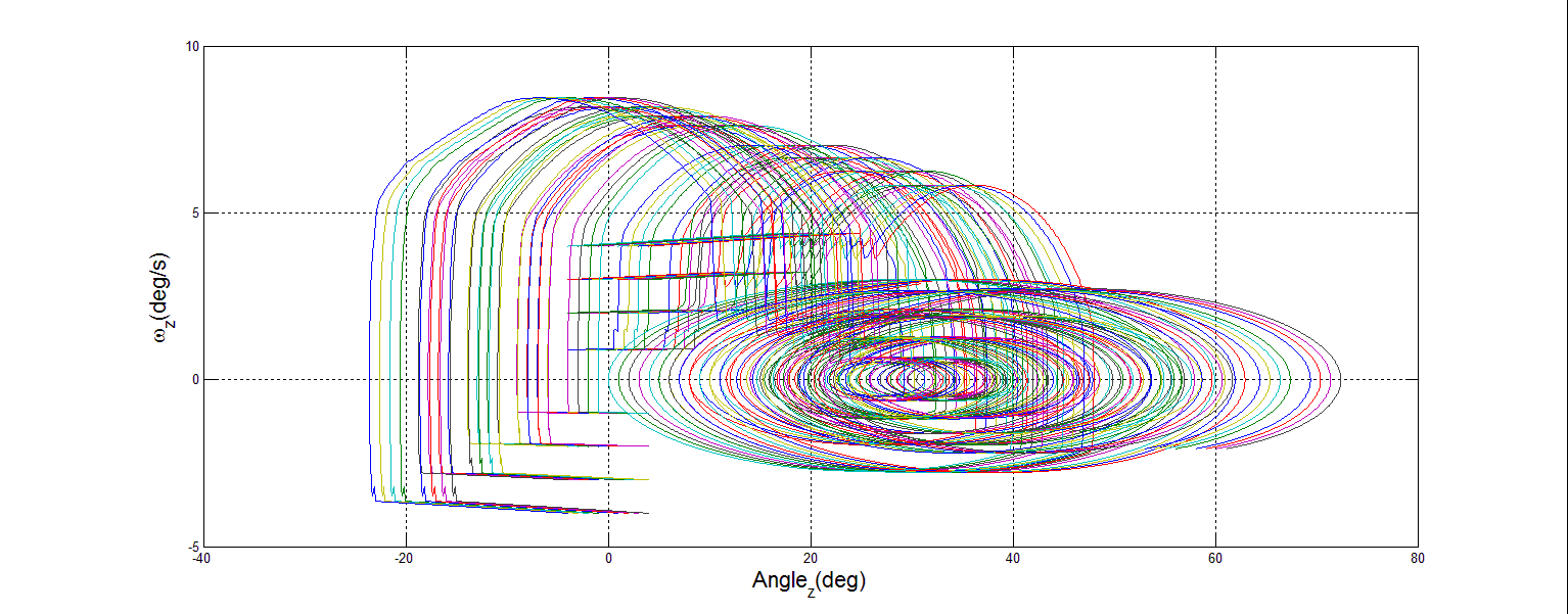 | Figure 25. 90% Mass Loss Z Phase Portrait |
4. Discussion
- The development of adaptive controls and the enabling technology for them has reached a point where new and innovative uses are now becoming possible. The purpose of this research was to determine the plausibility of DTC in satellites. By introducing a modified adaptive PID controller with adaptive feed forward control to this simulated spacecraft, it is demonstrated that the controls have achieved significant damage tolerance. This comes at a time where the need for such tools has never been greater, and the dangers associated with space operations grow daily.
4.1. Adaptive Control
- Space operations are going to become more difficult and dangerous in the foreseeable future. Significant action is required to protect the space assets that the United States has become dependent on. Adaptive control holds the key for many of the solutions currently proposed to mitigate these risks.The damage tolerant, adaptive controller as implemented in the simulation provides adaptive control with accuracy and stability. This accuracy is evidenced by Monte Carlo analysis where less than 1 degree of system tracking error even when approaching 90 percent mass loss. The stability is evidenced by the phase portraits of system performance in each inertial frame, recovering from the sudden change in state even when the change was accompanied by a loss of mass.
4.2. Application of Study
- Introducing DTC like those simulated here is achievable with today’s technology. As the largest limiting factor historically has been processing power, the feasibility of retrofitting operational spacecraft with DTC is limited, but not necessarily impossible. Modern spacecraft should have no technical limitations prohibiting the implementation of DTC. Writing DTC into spacecraft controllers may even lower the cost and risk of the program as a whole. [61] DTC clearly exhibits a stability solution for all manner of spacecraft, warranting further study and operational adoption. The logical next step is to validate the simulation results experimentally as done in [53-59, 63].Following experimental validation, military space missions [60] may be designed [61, 62] taking advantage of these developments.