1. Introduction

Analog electronic circuit fault diagnosis has gained wide spread attention in the area of atomised testing with the help of computers. Advances in the System on Chip technology have resulted in increased importance of the analog circuitry thus moving into the mainstream IC technology. The advances made in deep sub- micron technology and the co- existence of analog and digital circuits has increased the complexity of the IC’s. This has made fault diagnosis a very challenging task, particularly analog fault diagnosis.

There are two important fault diagnosis techniques which are based on the stage at which the simulation is carried out to test the system: Simulation After Test (SAT) and Simulation Before Test (SBT) approach.

In SAT approach the simulation is carried out at the time of testing. This is done to identify the Network parameters, by measuring the voltage and current. The faulty elements are then identified by determining those components which fall outside the design tolerance range.

The SBT approach places emphasis on building the fault dictionary, in which the nominal behaviour of the circuit in DC, Time domain or Frequency domain is stimulated. The responses of the circuit for various faults are stored in the fault dictionary. Fault simulation plays a very important role in the construction of the fault dictionaries. The factors that decide the effectiveness of this technique are the proper choice of stimulus, selection of test measurement optimization and fault isolation.

The number of test measurements is chosen such that all or maximum number of faults are diagnosed. This criterion may sometimes drastically increase the size of the fault dictionary. Optimisation is done to remove the measurements which are redundant or that do not help in fault isolation.

Mielke [1] introduced frequency domain analysis to test analog to digital converters using Fourier analysis. Wei et al [2] used large change sensitivity analysis to make optimum test point and test frequency selection. A hierarchical frequency domain robust component failure detection scheme was proposed by Sheu and Chang in [3].

Venu and Manasa [4] proposed multi frequency approach to fault diagnosis of analog circuits using pole sensitivity approach. Pinjala & Kim [5] presented an algorithm to select the optimum number of test points in frequency domain. The evaluation of algebraic indices was used by Grasso et al in [6] to select test frequencies. The algebraic invariant property of the transfer function has been used to present multi-frequency methods to diagnose faults by Swamy et al in [7]. Jantos et al [8] proposed heuristic methods to select the test frequency set. Alippi et al [9] addressed the problem of automatic selection of test frequencies by using global sensitivity analysis.

Slamani and Kaminska [10] presented a fault observability concept in the frequency domain analysis of analog circuits. Lavo and Larrabee [11] examined the various types of diagnosis data to reduce the size of the fault dictionaries. Babu and Prasad [12] proposed a method that uses RBFN neural networks to isolate faults in analog circuits. John W. Bandler and others [13] made an exhaustive and comprehensive review of different analog fault diagnosis methods. Baoru et al [14] proposed a diagnosis method for hard and soft faults using adoptive learning rate in BP neural networks.

Venu, Babu and Kishore [15] proposed a novel Node-Frequency approach using SBT approach to diagnose faults in analog circuits. Babu et al in [16] developed new algorithms which optimised the number of Frequencies needed to diagnose faults using SBT approach.

2. Test Frequency Selection Criterion

Seshu and Waxman [17] proposed an empirical procedure for the selection of test frequencies in linear electronic circuits. In this procedure the output for a certain magnitude of input is measured at different frequencies. Then the fault dictionary is constructed by calculating the gain of the system. The gain signatures are calculated for the nominal case and for all the selected faulty cases.

In this method the test frequencies are chosen such that there must be at least one frequency below the lowest non-zero break frequency and one between the successive break points. Also several test frequencies are to be selected near break points corresponding to complex critical frequencies. If the value of a parameter deviates from its nominal, the locations of poles and zeros also change. This consequently changes the magnitude of the transfer function. Some parameters change the location of more than one break point and measurement of gain at these frequencies gives different value of the magnitude.

The deviations of the parameter values from the nominal are called as faults, and the circuit is simulated for these faults along with the nominal values. The variation of the gain from the nominal is quantized and the gain signature is used in the construction of the fault dictionary.

The important phase in analog fault diagnosis using dictionary approach is the optimum selection of the test measurements. Optimum selection of test measurements involves only minimum number of measurements to diagnose maximum number of faults.

3. Integer Coded Fault Dictionary

The fault dictionary used in analog fault diagnosis is constructed by using different measurements of the circuit under test. The fault dictionary represents the readings of the circuit made under different fault conditions and one fault free condition. The measurements are made for a set of test frequencies (or test nodes) selected using any of the available criterions. The circuit parameters measured is generally the gain of the circuit under test.

Due to the inherent properties of the analog circuits, the measurements made are sometimes similar for different fault conditions or the values are very near to each other. This gives similar fault signatures for different faults, thus making fault diagnosis difficult. All those measured values which are either same or very close in range are termed as ambiguity sets, as these measurements lead to an ambiguous result.

For a circuit under test, there can be many ambiguity sets. To distinguish between these sets, integer codes are proposed by Lin and Elcherif [18]. They proposed a method in which the measurements are grouped and given integer numbers. These integer numbers indicate the ambiguity set to which the measurements belong. The fault dictionary measurements are now replaced by integer numbers, and the fault dictionary is now called as an integer coded fault dictionary.

The advantage of using an integer coded fault dictionary is that it gives a clear indication of the relation between the different fault signatures. Also an integer coded fault dictionary makes processing of data easy.

The integer coding is based on measurements which belong to certain range of similar values and taken at a particular node at different test frequencies. The ambiguity range is determined by taking the average value of the minimum and maximum values of the group. Next the range of deviation value is chosen tentatively. The integer coded fault dictionary provides information about the ambiguity sets for each test point, thus transforming the test frequency selection into the selection of columns to isolate rows.

4. Ambiguity Table Construction

Choose a Circuit Under Test (CUT) and simulate it for nominal and fault cases (either soft or hard faults). In the Multi Frequency approach, the test frequency is chosen as per the criterion mentioned in the earlier sections. The voltage gain is measured for different faults at all the chosen test frequencies. The fault signatures along with the nominal case are tabulated resulting in the fault dictionary.

The rows of the fault dictionary which denote fault signatures should be distinct, thus enabling diagnosis of all faults. But in general, some of the fault dictionary readings are either same or very near to each other, resulting in ambiguity in fault diagnosis. All these readings form ambiguity sets – set of faults which have almost the same fault signature.

The process of constructing the Ambiguity table is given in Procedure 1.

Procedure 1:

(a) Select a sensitivity range to define the ambiguity sets.

(b) Calculate the number of ambiguity sets for all frequencies in the test set.

(c) The faults are numbered sequentially starting from left and each fault is assigned with integer number that reflects the ambiguity group to which it belongs.

(d) If an ambiguity group consists of only one value, it is called a singleton.

(e) The fault dictionary is now replaced by integer values which reflect the ambiguity group to which they belong- Ambiguity Table.

(f) Finally, include the number of singletons (S) and total number of ambiguity sets (N) in the ambiguity table.

5. Optimum Selection of Frequencies Using Monte Carlo Analysis

In this paper the construction of a novel sub-ambiguity table using ambiguity table is proposed. The paper also proposes the use of sub-ambiguity sets to increase the number of faults diagnosed. The table that is constructed from an ambiguity table is called sub-ambiguity table. The principle behind the construction of the sub-ambiguity table is the reduction in sensitivity range which in turn is determined by the Monte Carlo simulations. The fault dictionary reduces the number of test measurements to be made thus reducing the size of the fault dictionary.

5.1. Algorithm 1

Step 1: Tabulate the ambiguity sets from the measurements made from the Circuit Under Test (CUT).

Step 2: Find out the number of singletons in all the rows of the table and select the row with the highest number of single tons.

Step 3: If there is more than one row having highest number of singletons, choose any one of them randomly. If the number of singletons is equal to total number of ambiguity sets then go to Step 9, else go to step 4.

Step 4: Intersect the rows chosen in Step 2 with the next highest singleton row, and see if more number of faults can be isolated. If not, go to step 5.

Step 5: Here the sub-ambiguity table is computed, using Monte Carlo Simulations (Using Algorithm 2).

Step 6: Repeat steps 3 and 4 to see if all the faults are eliminated. If yes go to step 8 else go to next step.

Step 7: The sub-ambiguity table can be constructed any numbers of times by further reducing the sensitivity range until all the faults are diagnosed or the desired number of faults are diagnosed. The sensitivity range limit of the circuit is determined by the Monte Carlo simulations for a certain pre-defined tolerance of the components.

Step 8: Stop.

5.2. Algorithm 2

This algorithm gives the procedure to construct an optimized sub ambiguity table.

Step 1: Start with a test frequency set that consists of only those frequencies which are not selected in Algorithm 1.

Step 2: Include only those faults which have not been identified in the earlier attempt.

Step 3: Run Monte Carlo analysis on the Analog System under Test (ASUT). Determine the maximum range of the measured values for faults for a pre-determined tolerance range.

Step 4: Use the value from Step 4 to decide the range of measured values to construct the sub-ambiguity table.

Step 5: Follow the steps in Algorithm- 1 for further fault diagnosis.

6. Illustration

Consider a fourth order Butterworth Anti-Aliasing filter shown in Figure 1. The transfer function H(s) of this circuit is given in Equation 1.

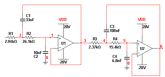Figure 1. Fourth order Butterworth Anti-Aliasing Filter

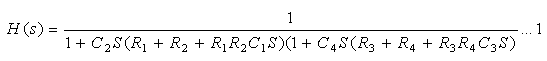The nominal component values of the circuit are R₁=2.94 KΩ, R₂=26.1KΩ, R₃=2.37KΩ, R₄=15.4KΩ, C₁=33nF, C₂=10nF, C₃=100nF and C₄=6.8nF. The break points of the network are at the corner frequencies 1000.16Hz and 1010.26Hz. The test frequencies chosen are f_T={ 750Hz (f₁), 800Hz (f₂), 900Hz (f₃), 950Hz (f₄), 1000Hz (f₅), 1005 Hz (f₆),1010 Hz (f₇) and 1200 Hz (f₈) }.

The illustration of the algorithm has been done taking only hard faults into consideration. Similarly the soft faults can also be considered. The faults considered are F₀=Nominal or Fault free, F₁=R₁ short, F₂=R₂ Short, F₃=R₃ Short, F₄=R₄Short, F₅=C₁ open, F₆= C₂ open, F₇=C₃ Open and F₈=C₄ Open. The voltage gain is measured at different faults and frequencies. The fault signatures are tabulated resulting in the fault dictionary shown in Table 1.

Table 1. Actual readings of the filter scaled by a factor ten

Based on the fault dictionary readings, the ambiguity sets are formed. The ambiguity sets are those sets of faults which have almost the same fault signature.

The range selected in this method is ± 0.2V. The ambiguity sets are shown in Figure 2. As seen from the Figure 2, the ambiguity sets are six for the first test frequency, six for second test frequency and so on. Also the sixth frequency (f₆) has a maximum number of singletons i.e., five out of a total number of nine faults. The ambiguity table constructed is based on the Figure 2.

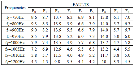
Figure 2. Ambiguity Sets

The total number of ambiguity sets is first found out from the figure shown in Figure 2. The faults are numbered sequentially starting from left and each fault is assigned with the integer number that reflects the ambiguity group to which it belongs to. For example for the first test frequency (f₁), faults F₃ and F₇ belong to the first ambiguity set and therefore the integer code is given as 1, similarly faults F₂ and F₆ are given the number 6 as they belong to the ambiguity set 6. Using this procedure the ambiguity table is constructed and is shown in Table 2, where ‘S’ is the number of singletons and ‘N’ is total number of ambiguity sets.

Table 2. Ambiguity Table Freq(Hz) FAULTS S(N) F0 F1 F2 F3 F4 F5 F6 F7 F8 f1 5 4 6 1 2 3 6 1 2 3(6) f2 5 4 6 1 2 3 6 1 2 3(6) f3 5 4 6 1 3 3 6 1 3 2(6) f4 5 4 6 1 2 3 6 1 2 3(6) f5 5 4 6 1 2 3 6 1 2 3(6) f6 5 4 6 1 2 3 7 1 2 5(7) f7 4 4 5 1 2 3 5 1 2 1(5) f8 2 2 3 1 2 2 3 1 2 0(3)

As per the step 2 of Algorithm 2, it is found from the Table 2 that the sixth frequency f₆=1005 Hz is having maximum number of singletons equal to 5. The frequency f₆ isolates 5 out of the total nine faults. Also using step 3 of the Algorithm 2, it is found that not all faults are isolated.

Now take the test frequency f₆ and intersect it with another test frequency (row) having the next highest number of singletons as per step 4. If this operation results in new faults being identified then choose this test frequency. The process is repeated to cover the whole frequency test set or till all the faults have been isolated. It has been found that the frequency f₆ =1005 Hz has isolated maximum number of faults. No other frequency from the test set is able to isolate faults apart from these. It has been found that the faults F₃, F₇, F₄ and F₈ are not isolated.

In the construction of the sub-ambiguity table, Monte Carlo analysis is carried out to identify the sensitivity range. The VLSI circuits now are fabricated with very low tolerances, and as such are highly precise. Here, Monte Carlo simulations have been done for 1% tolerance in all the components using Gaussian distribution.

Simulations have been carried out for ten runs and the maximum deviation from the nominal has been found to be 0.009mV in case of 1% tolerance (shown in Fig 3.4) and 0.05mV in case of 5% tolerance.

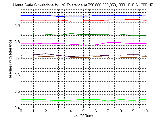Figure 3. Monte Carlo Simulations for 1% Tolerance

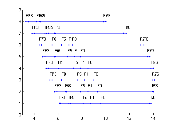
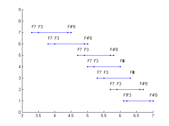Figure 4. Sub-Ambiguity Sets

The Components with 1% tolerance have been chosen and the sensitivity range is set to ±0.075V (from the earlier range of ±0.2 V) for achieving maximum fault isolation. The sub-ambiguity sets are shown in Figure 4. The sub-ambiguity table is constructed from Figure 4, and is shown in Table 3. As seen, the sub ambiguity table drastically reduces the size of the table resulting in a very fast implementation.

Table 3. Sub Ambiguity Table I”x FREQUENCIES FAULTS F3 F4 F7 F8 f1 2 3 1 4 f2 2 3 1 4 f3 2 3 1 3 f4 2 3 1 3 f5 2 3 1 4 f7 2 3 1 3 f8 2 3 1 4

From the Table 3, it is found that the frequencies f₃, f₄ and f₇ cannot be used as they do not isolate the desired faults, whereas all the other test frequencies f₁, f₂, f₅ or f₈ can be included in the optimized test frequency set. This is because they have ambiguity sets equal to the total number of faults. As all these frequencies isolate the faults, choose any one of these randomly. Thus the optimized test frequency set is (f₆, f₁). Complete fault isolation with two levels of ambiguity sets is achieved in the method presented in this section. This may not be the case always, but the endeavor is to achieve maximum fault isolation. The number of levels of ambiguity sets is only limited by the sensitivity range chosen.

7. Conclusions

In this paper various methods are proposed which not only reduce the number of test frequencies but also reduce the size of the fault dictionary. Monte Carlo analysis has been used to construct the sub-ambiguity table. For this the practical tolerances of the components are considered thus diagnosing more number of faults.