Rubén Villafuerte D.1, Rubén A. Villafuerte S.2, Jesús Medina C.3, Edgar Mejia S.3
1Department of Electrical Engineering, Faculty of Engineering, Universidad Veracruzana, Ciudad Mendoza Ver, 94724, Mexico
2Department of Electrical Engineering, Instituto Tecnologico de Orizaba, Orizaba, Ver, 94320, México
3Department of Mechanical Engineering, Faculty of Engineering, Universidad Veracruzana, Ciudad Mendoza Ver, 94724, Mexico
Correspondence to: Rubén Villafuerte D., Department of Electrical Engineering, Faculty of Engineering, Universidad Veracruzana, Ciudad Mendoza Ver, 94724, Mexico.
| Email: |  |
Copyright © 2012 Scientific & Academic Publishing. All Rights Reserved.
Abstract
This paper presents the results of applying different numerical methods for solving systems of nonlinear equations. Methods of three, four and five steps are used to solve the systems of nonlinear equations are generated when the behavior of electrical networks in steady state is analyzed. Specifically used to calculate the nodal voltages and know the flow of real and reactive power in a power grid. The results are compared with those reported in the literature and represent an improvement to those reported in[1].
Keywords:
Electrical Network, Iterative Methods, Nonlinear Equations, Nonlinear Systems, Power Flow, Voltage
Cite this paper: Rubén Villafuerte D., Rubén A. Villafuerte S., Jesús Medina C., Edgar Mejia S., New Methods for Solving Systems of Nonlinear Equations in Electrical Network Analysis, Electrical and Electronic Engineering, Vol. 4 No. 1, 2014, pp. 1-9. doi: 10.5923/j.eee.20140401.01.
1. Introduction
Numerical analysis in mathematics means to solve mathematical problems by arithmetic operations: addition, subtraction, multiplication, division and comparison. Since these operations are exactly those that computers can do, numerical analysis and computers are intimately related. With the development of fast, efficient digital computers, the role of numerical methods in solving scientific and engineering problems has increased dramatically in mode-time years. One of the most important problems in science and engineering is to find the solution of nonlinear equations. This problem is also termed as root finding problem. We know simple formulae for solving linear and quadratic equations and there are somewhat more complicated formulae for cubic and quartic equations, but not formulae like these are available for polynomial of degree greater four. Besides polynomial equations, there are many problems in scientific and engineering applications that involve the function of transcendental nature. Numerical methods are of often used to obtain approximated solution of such problems because it is not possible to obtain exact solution by usual algebraic processes.Newton method is probably the most widely used algorithm for finding simple roots, which stars with an initial approximation xo closer to the root α and generates a sequence of successive iterates  converging quadratically to simple to simple roots[2]. It is given by:
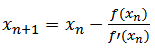 | (1) |
Many different derivations of Newton method are available in literature. We can say that at every iteration, we construct a local model of function f(x) at xn and solve for root xn+1.Newton's method is widely used in the calculation of the roots of non-linear equations, likewise, is used for solving nonlinear systems of equations, where the formation of the matrix of derivatives is essential in the solution. Solving a nonlinear equation, various methods have been proposed that use this method as a basis[3, 4, 5, 6]. For the solution of nonlinear equations system, most of the references utilize specialized matrix formulation, generating derived matrix known as the Jacobian, this is mainly due to the robustness posing and reflected by a small number of iterations in the iterative process.A significant number of methods have been proposed using various techniques, including quadrature formulas, Taylor series and decomposition techniques[7, 8, 9, 10]. King developed a fourth-order method are as follows[11].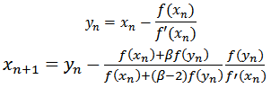 | (2) |
A three-step method and eighth order developed by Weihong Bi is as follows[12]: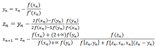 | (3) |
Linke Hou proposes a four-step method and twelfth order[13]: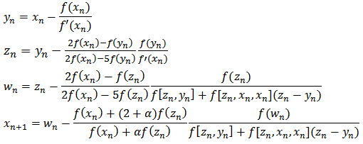 | (4) |
In many engineering applications, the values of the variables at each iteration are very close, in such cases it has been found that equations (3) and (4) or which involve the use of divided differences present some problems for convergence.In this study, we propose algorithms for two, three , four and five steps with which we can find the solution of a nonlinear equation, also, we have used the same algorithms for solving systems of nonlinear equations, without having to form the matrix of derivatives that have been proposed by other authors[14].
2. Proposed Methods for Solving Nonlinear Equations and Systems of Nonlinear Equations
For the solution of nonlinear equations and systems of nonlinear equations, we propose the methods described below.Two-Step Method (M12P)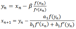 | (5) |
Three-step method (M13P):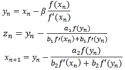 | (6) |
Three-step method (M23P): 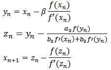 | (7) |
Where: a1, a2, a3, b1, b2, b3, are real numbers.Four-step method (M14P):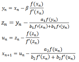 | (8) |
Five-step method (M15P):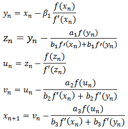 | (9) |
Where: a1, a2, a3, b1, b2, b3,  , are real numbers.In equations (5) to (9), ßi is considered[15], as a multiplicity factor, in the results reported in this paper shows the importance of this issue in solving systems of nonlinear equations[16].
3. Systems of Nonlinear Equations
Consider the system of n nonlinear equations of the form: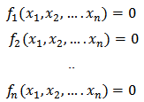 | (10) |
We denote Rn the real n-dimensional space of column vectors with components x1, x2, .. xn. Each function fi can be thought of as mapping a vector (x1, x2... xn)t of the n-dimensional space Rn into the real R. The elements of Rn are called vectors. We use the following notations (boldface letters) to denote vectors: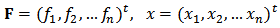 This system of nonlinear equations in n unknowns can be represented by defining a function F mapping Rn into Rn as:
 | (11) |
Thus equation (11) becomes: | (12) |
The functions 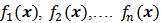 are de coordinated functions of
  . The derivative
  y
y  is called first Fréchet derivative. The matrix representation of
  is given by the Jacobian matrix denoted by
  and is given by:
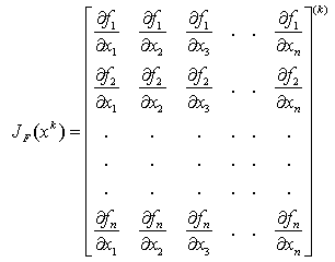 | (13) |
If we solve a system of nonlinear equations in matrix form the matrix formation is required, and Newton's method is equal to: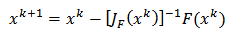 | (14) |
In the solution of systems of nonlinear equations[16] proposes, among others, the following method: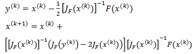 Methods: (M12P), (m13p) and (M14P), proposed by the authors for solving nonlinear systems of equations can be expressed in matrix form as follows:
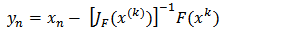 | (15) |
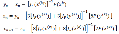 | (16) |
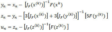 | (17) |
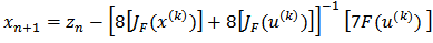 | (18) |
Evaluating the partial derivative matrix JF(x(k)), and JF(y(k)), are required at each step of the iterative process. A two-step method and fourth-order developed by Cordero to solve a system of nonlinear equations[17]: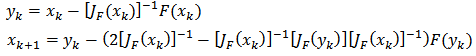 | (19) |
Another method also developed by Cordero of three steps and sixth order is as follows[18]: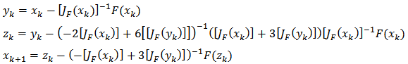 | (20) |
4. Results
Four cases have been selected where systems are represented by grids nonlinear equations; the solution is obtained by applying the methods (5) to (9). In each case, it is not necessary to form the Jacobian matrix for the solution of the equation system.Case 1.In[19] we have a set of four nonlinear equations, which is shown in Figure 1, and by network conditions only three equations are solved. | Figure 1. Four-node Network[19] |
In Tables 1 and 2 respectively show the characteristics of the network which generates the functions represented by equation (11), to solve the system of nonlinear equations (12).| Table 1. System data in Figure 1 |
| | Line (Lij) | Impedance | Admitance | | 1-2 | 0.01008+j0.5040 | j0.05125 | | 1-3 | 0.00744+j0.03720 | J0.03875 | | 2-4 | 0.0744+j0.03720 | J0.03875 | | 3-4 | 0.01272+j0.06360 | J0.06375 |
|
|
| Table 2. Data system of Figure 1 |
| | Node | Sgen | Sload | V(o) | Node Type | | 1 | 0+j0 | 50+j30.99 | 1.00+j0 | Slack | | 2 | 0+j0 | 170+j105.35 | 1.00+j0 | Load | | 3 | 1.0+jQ | 200+j123.94 | 1.00+j0 | Load | | 4 | 318+jQ | 80+j49.58 | 1.02+j0 | V. Controlled |
|
|
Case 2.In reference[20], generates a set of five non-linear equations, which is shown in Figure 2, by the characteristics of the network are solved only four.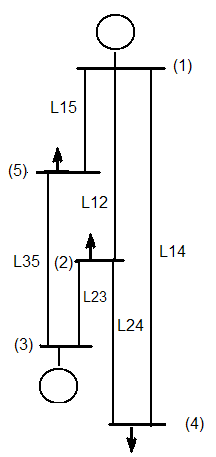 | Figure 2. Five-node system[20] |
In Tables 3 and 4, respectively, we show the characteristics of the network which generates the functions represented by equation (11), to solve the system of nonlinear equations (12).| Table 3. System data in Figure 2 |
| | Line (Lij) | Impedance | | 1-2 | 0.10+j0.40 | | 1-4 | 0.15+j0.60 | | 1-5 | 0.05+j0.20 | | 2-3 | 0.05+j0.20 | | 2-4 | 0.10+j0.40 | | 3-5 | 0.05+j0.20 |
|
|
| Table 4. Data network operation |
| | Node | Sgen | Sload | V(o) | Node Type | | 1 | 0+j0 | 0+j0 | 1.02+j0.0 | Slack | | 2 | 0+j0 | 0.6+j0.3 | 1.0+j0 | Carga | | 3 | 1.0+jQ | 0+j0 | 1.04+ja | V. Controlled | | 4 | 0+j0 | 0.4+j0.1 | 1.0+j0 | Load | | 5 | 0+j0 | 0.6+j0.2 | 1.0+j0 | Load |
|
|
Case 3.In[21], there are a set of five non-linear equations, and as shown in Figure 1, for network conditions only four equations are solved.Complete system data are shown in Tables 5 and 6.| Table 5. System data in Figure 3 |
| | Line (Lij) | Impedance | Admitance | | 1-2 | 0.02+j0.06 | j0.030 | | 1-3 | 0.08+j0.24 | j0.025 | | 2-3 | 0.06+j0.18 | j0.020 | | 2-4 | 0.06+j0.18 | j0.020 | | 2-5 | 0.04+j0.12 | j0.015 | | 3-4 | 0.01+j0.03 | j0.010 | | 4-5 | 0.08+j0.24 | j0.025 |
|
|
| Table 6. Data network operation |
| | Node | Sgen | Sload | V(o) | Node Type | | 1 | 0+j0 | 0+j0 | 1.06+j0.0 | Slack | | 2 | 0.4+jQ | 0.2+j0.1 | 1.045+j0 | V. Controlled | | 3 | 0.3+jQ | 0.2+j0.15 | 1.03+ja | V. Controlled | | 4 | 0+j0 | 0.5+j0.3 | 1.0+j0 | Load | | 5 | 0+j0 | 0.6+j0.4 | 1.0+j0 | Load |
|
|
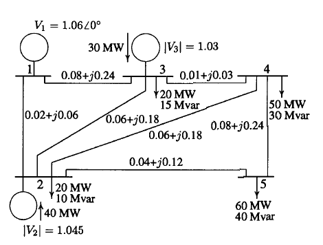 | Figure 3. Five-node system (21) |
Case 4.In[22], we can generate a system of nine non-linear equations, which is shown in Figure 4, for network conditions are resolved only eight nonlinear equations.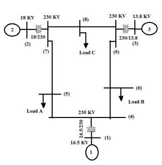 | Figure 4. Nine nodes system (22) |
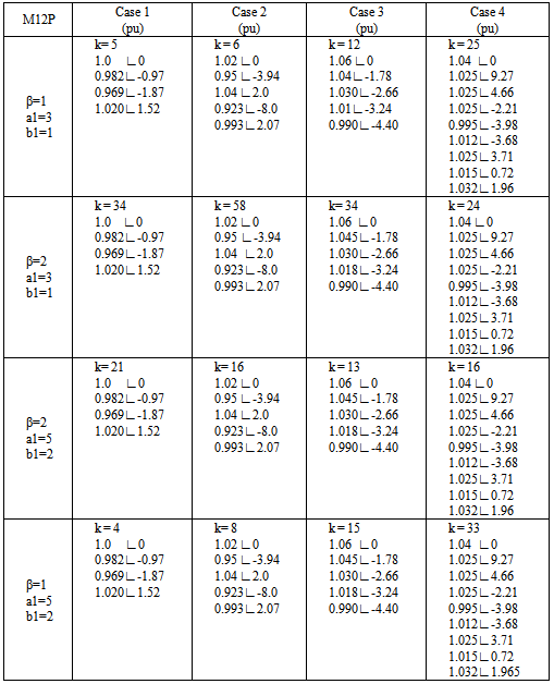
The results obtained with the method (M12P) in two steps in the four cases are shown in Table 7.Table 7. Results with the method M12P
 |
| |
|
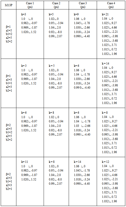
The results obtained with the method (M13P) of three steps in the four cases are shown in Table 8.Table 8. Results with the three-step method M13P
 |
| |
|
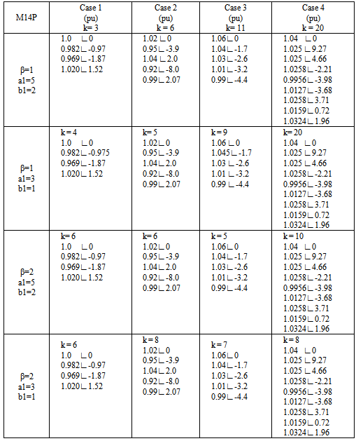
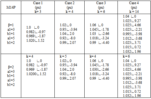
The results obtained with the method (M14P) of four steps in the four cases are shown in Tables 9 and 10.Table 9. Results with the four-step method M14P
 |
| |
|
Table 10. Results with the four-step method M14P
 |
| |
|
The five-step method is also applicable to each of the cases, and the results are shown in Table 11.Table 11. Results with the method M15P
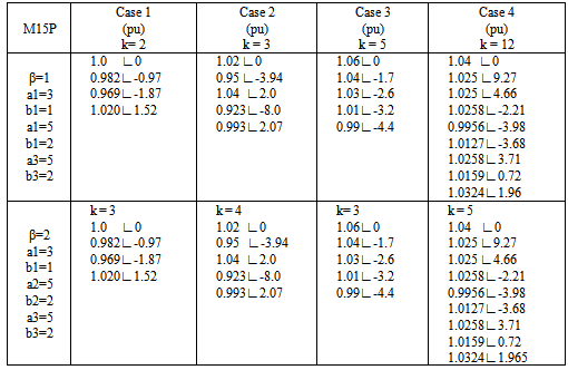 |
| |
|
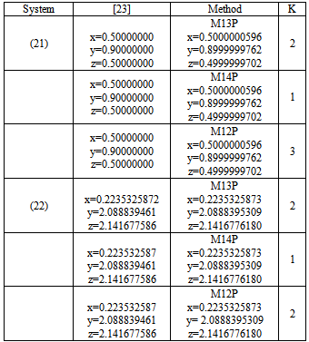
Systems of nonlinear equations shown below to be solved with the equations (16), (17) and (18).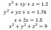 | (21) |
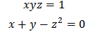 | (22) |
Table 12 shows the values obtained for each of the variables in equations (21) and (22).Table 12. Value of a root system (21) and (22)
 |
| |
|
5. Conclusions
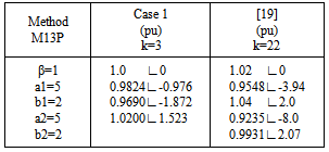
The proposed methods we apply to the solution of the nonlinear equations of electrical networks operating in steady state, specifically, to calculate the voltage at each node of a power system and power flow in transmission lines. The results are very consistent with those reported in books and literature that we have taken as reference[19, 20, 21, 22].The differences between the values that we obtain and those reported in references[19, 20, 21, 22] are not important, however, with respect to the formulation, if there are significant differences, especially when Newton's method is used in matrix form. In those methods, the matrix formulation using the number of iterations is generally less than 5, but the establishment of the Jacobian matrix is perhaps the main disadvantage. In the methods that we used, not create the matrix of derivatives, for this reason which increases the number of iterations, however, as you can see in the tables shown above, these methods are not demanding in the formulation and get them comparable with values from the references. Equations (21) and (22), we try to solve by applying the same formula that was used to solve the nonlinear equations of power grids, this in order to simplify the solution process, however, the results that we found no were adequate, for this reason methods are proposed (16), (17) and (18) in matrix form.The values in the third column of Table 12, we got them we develop programs in Visual Fortran, you can see on the same table the differences in values and may approach more if accuracy if tolerance is reduced, affecting possibly in one or more iterations in the solution. The methods we proposed, also developed in Visual Fortran, preserving in all cases a tolerance of 1.0e-10.In summary, we have proposed three methods for solving nonlinear equations in the plane where Cn is not necessary to form the Jacobian matrix at the same time, we have proposed methods for solving systems of nonlinear equations in Rn. To ensure accuracy, the proposed methods for solving systems of nonlinear equations forming the Jacobian matrix is needed, however as we can see in table 13, the number of iterations is small.Table 13. Results method M13P and reference[19]
 |
| |
|
References
| [1] | Rubén Villafuerte D., Rubén A. Villafuerte Salcedo, Jesús Medina C., Edgar Mejía S. “Multi-Step Methods Applied to Nonlinear Equations of Power Networks”, Scientific & Academic Publishing, Electrical and Electronic Engineering 2013, 3(5):128-132. |
| [2] | Chi Chun-Mei and Feng Gao, “A Few Numerical Methods for Solving Nonlinear Equations”, International Mathematical Forum, 3, 2008, no 29, 1437-1443. |
| [3] | Muhammand Rafiullah, “Three-Step Iterative Method with Sixth Order Convergence for Solving Nonlinear Equations”, International Journal of Math. Analysis, Vol. 4, 2010, no 50, 2459-2463. |
| [4] | Zhong LI, Chensong PENG, Tianhe ZHOU, Jun GAO, “A New Newton-type Method for Solving Nonlinear Equations with Any Integer Order of Convergence”, Journal of Computational Information Systems 7: 7(2011) 2371-2378. |
| [5] | S. Weerakoon and T. G. I. Fernando, “A variant of Newton´s Method with Accelerated Third-Order Convergence”, Applied Mathematics Letters 13 (2000) 87-93. |
| [6] | Fazlollah Soleymani, S. Karimi Vanini, Hani I. Siyam, and I. A. AI-Subaihi, “Numerical solution of equations by an optimal eighth-order of iterative methods”, Ann Univ Ferrara (2013) 59:159-171. |
| [7] | Cordero A., Hueso, J. L., Martínez, E. Terregosa J. R., “A Modified Newton-Jarrat’s Composition”, Numerical Algorithm, 55 (2010), 87-99. |
| [8] | Hueso J. l., Martínez E., Terregrosa, J. R., “Third order iterative Methods free from second derivative for nonlinear systems”, Applied mathematics and Computation, 211 (2009), 190-197. |
| [9] | Liang F. and Gouping He, “Some Modifications of Newton’s Method With Higher-order Convergence for Solving Nonlinear Equations”, Journal of Computational and Applied Mathematics 228(2008) 296-303. |
| [10] | Tetsuro Yamamoto, “Historical developments in convergence analysis for Newton’s and Newton-like methods”, Journal of Computational and Applied Mathematics 124 (2000), 1-23. |
| [11] | R. F. King, “A family of fourth order methods for nonlinear equations”, SIAM J. Numer. Anal. 10(1973) 876-879. |
| [12] | Weihong Bi, Hongmin Ren, and Qingbiao Wu, “Three-step iterative methods with eighth-order convergence for solving nonlinear equations”, Journal of Computational and Applied Mathematics 225 (2009) 105-112. |
| [13] | Linke Hou and Xiaowu Li, “Twelfth-order Method for Nonlinear Equations”, IJRRAS 3(1) April 2010. |
| [14] | M. A. Hafiz and Mohamed S. M. Bahgat, “An Efficient Two-step Iterative Method for Solving System Nonlinear Equations”, Journal of Mathematics Research, Vol. 4, No 4; 2012. |
| [15] | Bruno Salvy, “Numerical Elimination, Newton Method and Multiple Roots”, F. Chyzak INRIA 82003), 49-54. |
| [16] | Janak Raj Sharma and Rajni Sharma, “Some Third Order Methods for Solving Systems of Nonlinear Equations”, World of Science, Engineering and technology 60, 2011. |
| [17] | Cordero A, Martínez. Hueso, J. L. Martínez E. and Torregrosa, J. R., A “Modified Newton-Jarrat´s Composition”, Number Algo (55) 2010, 87-99. |
| [18] | Cordero A, Martínez, E. and Torregrosa, J. R. “Iterative Methods of Order Four and Five for Systems of Nonlinear Equations”, Appl. Math. Comput. 231(2009); 541-551. |
| [19] | J. J. Grainger and W. D. Stevenson Jr, “Análisis de sistemas de potencia”, McGraw-Hill, 1996. |
| [20] | W. D. Stevenson, “Análisis de sistemas de potencia”, McGraw-Hill, 1975. |
| [21] | Saadat H. , “Power Systems Analysis”, 2a edition, 2004. |
| [22] | P. M. Anderson & A. A. Fouad, “Power System Control and stability”, 2nd edition IEEE Press Power Engineering Series, Wiley-Interscience, 2003. |
 Abstract
 Reference
 Full-Text PDF
 Full-text HTML