-
Paper Information
- Next Paper
- Previous Paper
- Paper Submission
-
Journal Information
- About This Journal
- Editorial Board
- Current Issue
- Archive
- Author Guidelines
- Contact Us
Electrical and Electronic Engineering
p-ISSN: 2162-9455 e-ISSN: 2162-8459
2013; 3(2): 49-71
doi:10.5923/j.eee.20130302.04
Investigation of Nigerian 330 kV Electrical Network with Distributed Generation Penetration – Part I: Basic Analyses
 Abstract
 Reference
 Full-Text PDF
 Full-text HTML
Funso K. ARIYO, Micheal O. Omoigui
Department of Electronic and Electrical Engineering, Obafemi Awolowo University, Ile-Ife, Nigeria
Correspondence to: Funso K. ARIYO, Department of Electronic and Electrical Engineering, Obafemi Awolowo University, Ile-Ife, Nigeria.
| Email: |  |
Copyright © 2012 Scientific & Academic Publishing. All Rights Reserved.
The first part of this paper presents the basic analyses carried out on Nigerian 330 kV electrical network with distributed generation (DG) penetration. The analyses include load flow, short circuit, transient stability, modal/eigenvalues calculation and harmonics. The proposed network is an expanded network of the present network incorporating wind, solar and small-hydro sources. The choice of some locations of distributed generation has been proposed by energy commission of Nigeria (ECN). The conventional sources and distributed generation were modeled using a calculation program called PowerFactory, written by DIgSILENT.
Keywords: Distributed generation, load flow, short-circuit, transient stability, modal analysis, eigenvalues calculation, harmonics analysis, PowerFactory, DIgSILENT
Cite this paper: Funso K. ARIYO, Micheal O. Omoigui, Investigation of Nigerian 330 kV Electrical Network with Distributed Generation Penetration – Part I: Basic Analyses, Electrical and Electronic Engineering, Vol. 3 No. 2, 2013, pp. 49-71. doi: 10.5923/j.eee.20130302.04.
Article Outline
1. Introduction
- Nigeria is a vast country with a total of 356, 667 sq miles (923,768 km2), of which 351,649 sq. miles (910,771 sq km or 98.6% of total area) is land. The nation is made up of six geo-political zones subdivided into 36 states and the Federal Capital Territory (F.C.T.). Furthermore, the vegetation cover, physical features and land terrain in the nation vary from flat open savannah in the North to thick rain forests in the south, with numerous rivers, lakes and mountains scattered all over the country with population of 162,470,737 Million people. The total installed capacity of the currently generating plants is 7,876 MW, but the available capacity is around 4,000 MW with peak value of 4,477.7 MW on 15th August 2012. Seven of the fourteen generation stations are over 20 years old and the average daily power generation is below 4,000 MW, which is far below the peak load forecast of 8,900MW for the currently existing infrastructure. As a result, the nation experiences massive load shedding [1-5]. This paper looks at the conventional energy generation as well as the distributed generation sources: small-hydro, solar and wind energy potentials in Nigeria. The solar, small-hydro and wind energies are ways of accelerating the sluggish nature of the federal government of Nigeria rural electrification programmes. Nigeria receives an average solar radiation of about 7.0kWh/m2-day in the far north and about 3.5kWh/m2-day in the coastal latitudes [6]. Wave and tidal energy is about 150,000 TJ/year and the highest average speeds of about 3.5 m/s and 7.5 m/s in the south and north areas respectively [7-10]. Wind energy generating stations were proposed in the Northern part of the Country and along the coast in the southern part where average wind speeds are high, while solar stations were proposed for every state, having potentials to produce energy from the sun because of high solar radiation (minimum value of 50 MW per state). Offshore wind power was proposed for states along the coast which include: Lagos, Ondo, Delta, Bayelsa, and Akwa-Ibom (minimum value of 50 MW per state). It involves the construction of wind farms in bodies of water to generate electricity from wind. Better wind speeds are available offshore compared to on land, so offshore wind power’s contribution in terms of electricity supplied is higher. However, offshore wind farms are relatively expensive. This proposition coupled with ECN investigated sites were used to prepare the proposed electrical network for the Country (37-bus system) as shown in Figure 1, the power generation and allocation are shown in Table 1 (Appendix).However, penetration of DG can affect the stability of the system by either improving or deteriorating the stability of the system. The power system faces many problems when distributed generation is added in the already existing system. The addition of generation could influence power quality problems, degradation in system reliability, reduction in the efficiency, over voltages and safety issues [11-13].
2. Methodology
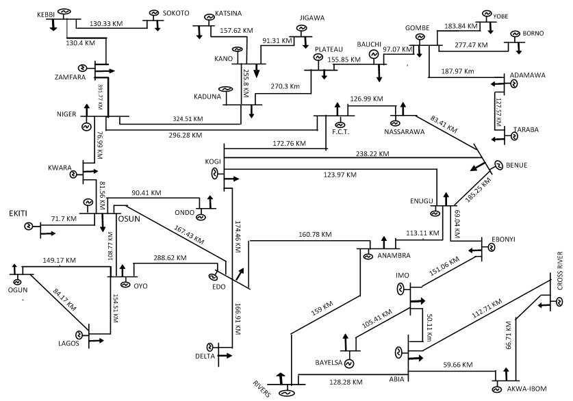 | Figure 1. Proposed Nigerian 330 kV electrical network (37-bus system) |
3. Network Modeling in PowerFactory
- The network model contains the electrical and graphical information for the grid. To further enhance manageability, this information is split into two subfolders: diagrams and network data. An additional subfolder, Variations, contains all expansion stages for planning purposes. The network model folder contains the all graphical and electrical data which defines the networks and the single line diagrams of the power system under study. This set of data is referred as the network data model. The proposed Nigerian 330 kV electrical network (37 buses), shown in Figure 1.0, was modelled using this software. The DGs are limited to solar, small-hydro and wind sources. The elements data used to carry out PowerFactory analyses are shown in Appendix. The base apparent power
 used is 100 MVA, while the transmission line lengths (in Kilometers, Km) were per-unitized on the base value of 100 Km.
4. Load Flow Analysis
- In PowerFactory, the nodal equations used to represent the analyzed networks are implemented using two different formulations:• Newton-Raphson (current equations)• Newton-Raphson (power equations, classical)In both formulations, the resulting non-linear equation systems are solved by an iterative method. Load flow calculations are used to analyze power systems under steady-state and non-faulted (short-circuit-free) conditions. The load flow calculates the active and reactive power flows for all branches, and the voltage magnitude and phase for all nodes under A.C. balanced, A.C. unbalanced and D.C. load flow calculation methods. The machine currents at steady-state are calculated from [15]:
 | (1) |
 is the terminal voltage of the ith generator; and
 and
and  are the generator real and reactive powers.For n-bus system, the node-voltage equation in matrix form is:
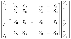 | (2) |
 | (3) |
 is the vector of the injected bus currents and
  is the vector of bus voltages measured from the reference node.
  is known as the bus admittance matrix. The diagonal element of each node is the sum of admittances connected to it. It is known as self-admittance given as:
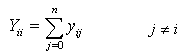 | (4) |
 | (5) |
 of the nodes, and the active (P) and reactive (Q) power flow on branches. The network nodes are represented by specifying two of these four quantities. PowerFactory uses the Newton-Raphson (power equation, classical) method as its non-linear equation solver. This method is used for large transmission systems, especially when heavily loaded. It was used for A.C. load flow.From Kirchhoff’s Current law (KCL), the current at bus I is given by [7]:
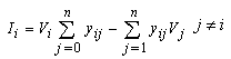 | (6) |
 | (7) |
 | (8) |
 | (9) |
 | (10) |
 and
and  , the voltage and phase angle for each bus are computed iteratively using:
 | (11) |
 and
and  are calculated from Jacobian matrix. The results of the analysis are shown and discussed in section 9.
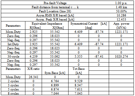
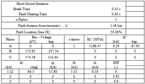
5. Short-Circuit Analysis
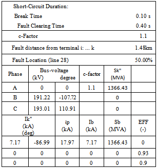
- The short-circuit calculation in PowerFactory is able to simulate single faults as well as multiple faults of almost unlimited complexity. As short-circuit calculations can be used for a variety of purposes, PowerFactory supports different representations and calculation (IEC60906, VCE0102, ANSI and complete) methods for the analysis of short-circuit currents. One application of short-circuit calculations is to check the ratings of network equipment during the planning stage. This is used in determining the expected maximum currents (for the correct sizing of components) and the minimum currents (to design the protection scheme). A single phase ‘a’ to ground was introduced on a transmission line linking Niger and F.C.T. generating stations using IEC60906 and ANSI methods, results are discussed in section 9 [16,17].
6. Transient Analysis
- The transient simulation functions available in DIgSILENT PowerFactory are able to analyze the dynamic behavior of small systems and large power systems in the time domain. These functions therefore make it possible to model complex systems such as industrial networks and large transmission grids in detail, taking into account electrical and mechanical parameters. Transients, stability problems and control problems are important considerations during the planning, design and operation of modern power systems. Short circuit switching events were created on transmission line linking Niger and F.C.T. generating stations, Benue, Sokoto, Kebbi, Borno generating stations, and loss of Rivers state load. These are transient faults carried out using electromechanical transients simulation method in PowerFactory software [11-13, 17-20].
7. Eigenvalues/Modal Analysis
- The modal analysis calculates the eigenvalues and eigenvectors of a dynamic multi-machine system including all controllers (defined before transient analysis) and power plant models. This calculation can be performed not only at the beginning of a transient simulation but also at every time step when the simulation is stopped. The eigenvalue analysis allows for the computation of modal sensitivities with respect to generator or power plant controllers, reactive compensation or any other equipment. The calculation of eigenvalues and eigenvectors is the most powerful tool for oscillatory stability studies. Starting from these ’bare natural’ modes, the effects of controllers (structure, gain, time constants etc.) and other additional models can be calculated as the second step [14]. One of the conjugate complex pair of eigenvalues is given by:
 | (12) |

 The period and damping of this mode are given by:
 | (13) |
 | (14) |
 and
and  are amplitudes of two consecutive swing maxima or minima respectively.The oscillatory periods of local generator oscillations are typically in the range of 0.5 to 5 Hz. Higher frequencies of the natural oscillations, that is, those which are normally not regulated out, are often damped to a greater extent than slower oscillations. The oscillatory period of the oscillations of areas (inter-area oscillations) is normally a factor of 5 to 20 times greater than that of the local generator oscillations [14].The absolute contribution of an individual generator to the oscillation mode which has been excited as a result of a disturbance can be calculated by:The nomenclature is given in Appendix.‘c’ is set to the unit vector, that is, c = [1, ...,1], which corresponds to a theoretical disturbance which would equally excite all generators with all natural resonance frequencies simultaneously. The elements of the eigenvectors
  then represents the mode shape of the eigenvalue i and shows the relative activity of a state variable, when a particular mode is excited. They show for example, the speed amplitudes of the generators when an eigenfrequency is excited, whereby those generators with opposite signs in
  oscillate in opposite phase. The right eigenvectors
  can thus be termed the "observability vectors''. The left eigenvectors
  measures the activity of a state variable x in the i-th mode, thus the left eigenvectors can be termed the "relative contribution vectors''. Normalization is performed by assigning the generator with the greatest amplitude contribution the relative contribution factor 1 or -1 respectively. For n-machine power system, n-1 generator oscillation modes will exist and n-1 conjugate complex pairs of eigenvalues
  will be found. The mechanical speed
  of the n generators will then be described by [14]:
 | (15) |
 and
and  are combined to a matrix P of participation factor by:
 | (16) |
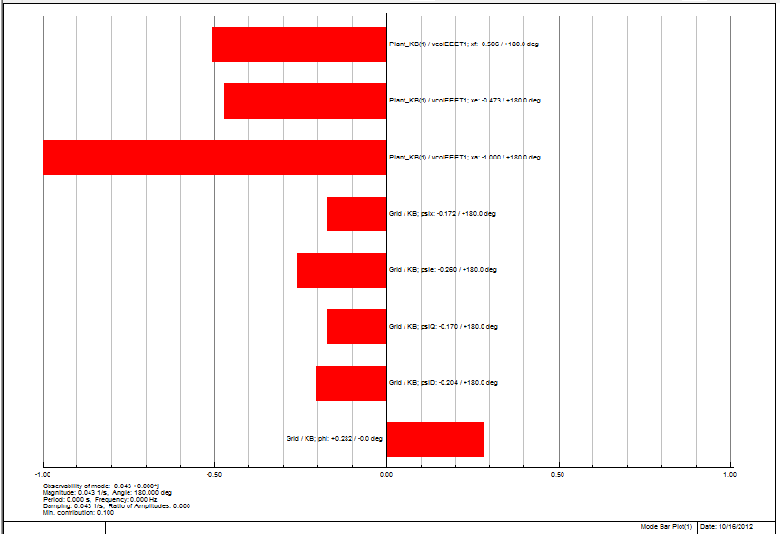
 are called the participation factors. They give a good indication of the general system dynamic oscillation pattern. They may be used easily to determine the location of eventually needed stabilizing devices in order to influence the system damping efficiently. Furthermore the participation factor is normalized so that the sum for any mode is equal to 1[21, 22].
8. Harmonics Analysis
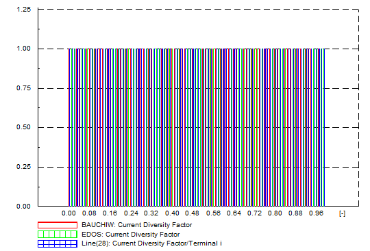
- One of several aspects of power quality is the harmonic content of voltages and currents. Harmonics can be analyzed in either the frequency domain, or in the time-domain with post-processing using Fourier analysis. The PowerFactory harmonics functions allow the analysis of harmonics in the frequency domain, it could be used to analyse both balanced and unbalanced network. Two different functions are provided by PowerFactory [14]:• Harmonic load flow;• Frequency sweep.In the case of a symmetrical network and balanced harmonic sources, characteristic harmonics either appear in the negative sequence component (5th, 11th, 19th, etc.), or in the positive sequence component. Hence, at all frequencies a single-phase equivalent (positive or negative sequence) are used for the analysis, while for analyzing non-characteristic harmonics (3rd-order, even-order, inter-harmonics), or harmonics in non-symmetrical networks, the unbalanced option for modeling the network in the phase-domain is selected.Frequency sweep is used to calculate frequency dependent impedances, the impedance characteristic can be computed for a given frequency range using ComFsweep in PowerFactory [14]. Harmonic analysis by frequency sweep is used for analyzing self- and mutual- network impedances. The voltage source models available in PowerFactory allow the definition of any spectral density function. Hence, impulse or step responses of any variable can be calculated in the frequency domain. Balanced, positive sequence uses a single-phase, positive sequence network representation, valid for balanced symmetrical networks. A balanced representation of unbalanced objects is used, while unbalanced, 3 Phase (ABC) uses a full multiple-phase, unbalanced network representation.The second function is the frequency sweep performed for the frequency range defined by the ‘Start Frequency’ and the ‘Stop Frequency’, using the given Step Size. An option is available which allows an adaptive step size. Enabling this option will normally speed up the impedance calculation, and enhance the level of detail in the results by automatically using a smaller step size when required [23, 24].
9. Results and Discussion
|
|
|
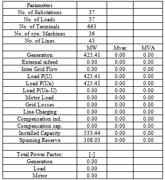
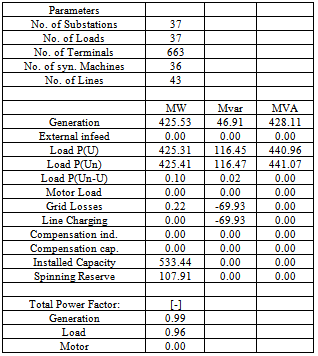
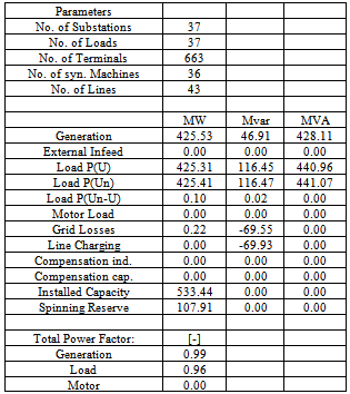
 used was 100 MVA, while the transmission line lengths (in Kilometers, Km) were per-unitized on the base value of 100 Km.Detailed reports can be provided in the ‘output of results-complete system report’ icon provided by the software.Secondly, short-circuit calculation was carried out on transmission line connecting F.C.T. and Niger generating stations.
|
|
|
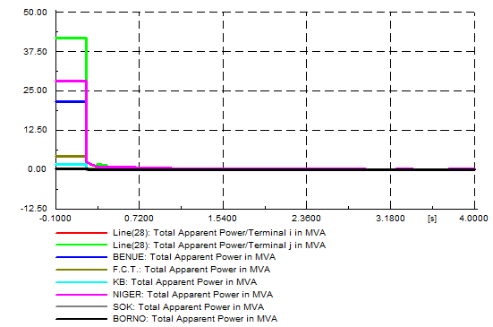 | Figure 2. Total apparent power (MVA) |
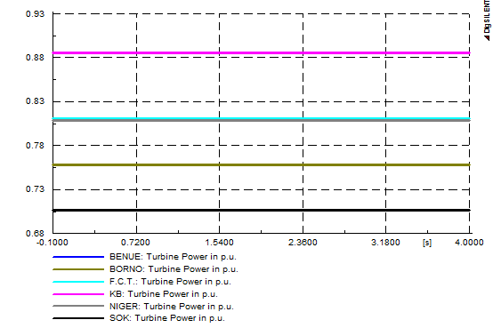 | Figure 3. Turbine power (p.u.) |
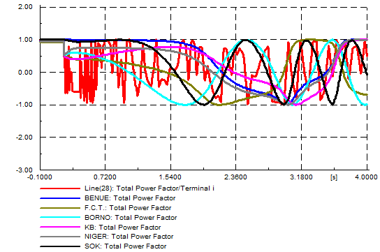 | Figure 4. Total power factor |
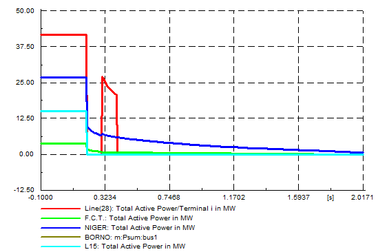 | Figure 5. Total active power (MW) |
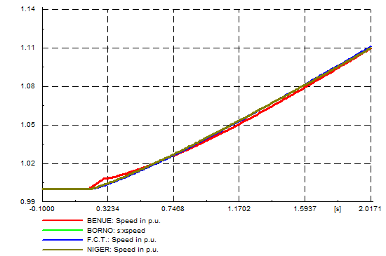 | Figure 6. Speed (p.u.) |
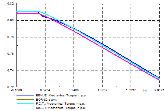 | Figure 7. Mechanical torque (p.u.) |
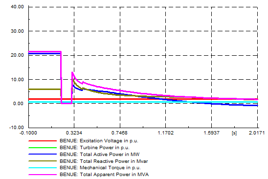 | Figure 8. Benue hydro generating station parameters |
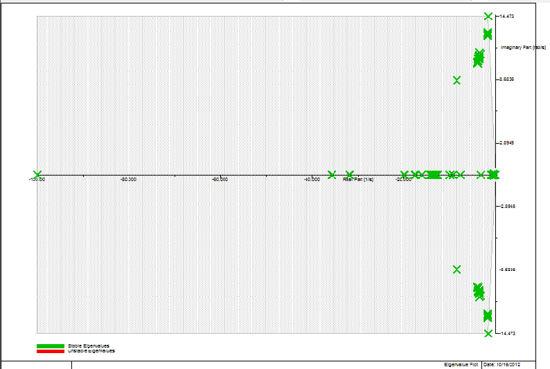 | Figure 9. Eigenvalue plot – QR method |
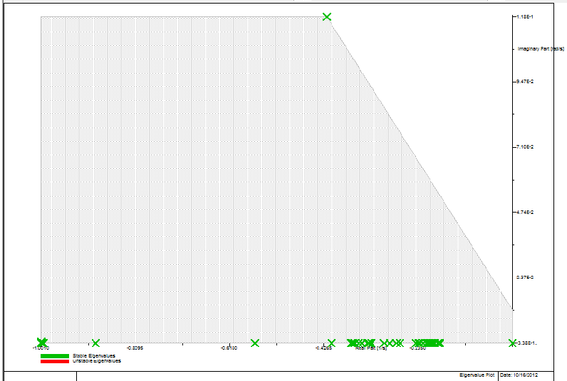 | Figure 10. Eigenvalue plot - selective method |
 | Figure 11. Mode bar plot - controllability |
 | Figure 12. Mode bar plot - observability |
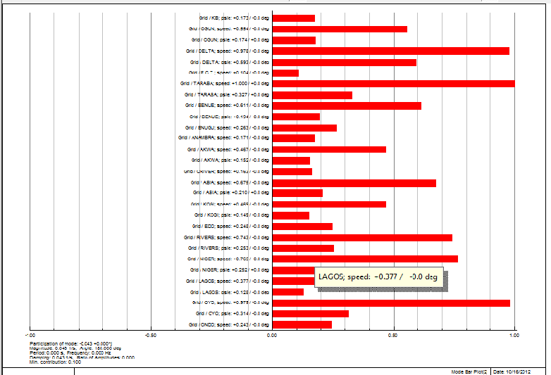 | Figure 13. Mode bar plot - participation factor |
 | Figure 14. Mode phasor plot - controllability (0,0 origin) |
 | Figure 15. Mode phasor plot - observability (0,0 origin) |
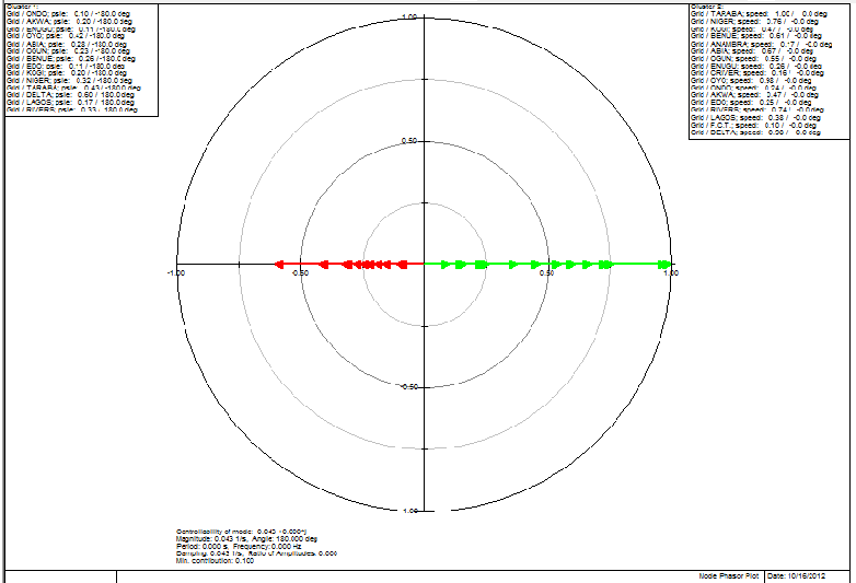
 | Figure 16. Mode phasor plot - participation factor |
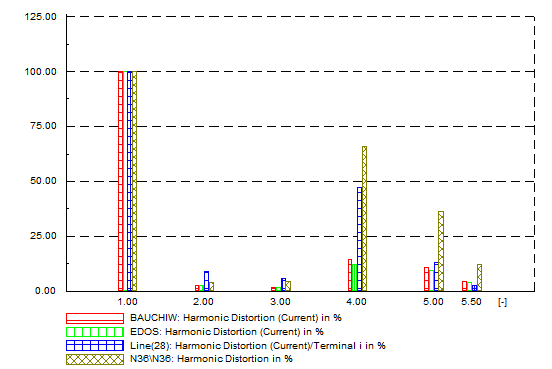 | Figure 17. Balanced network - harmonic distortion, A |
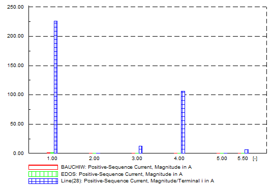 | Figure 18. Balanced network - positive-sequence current, A |
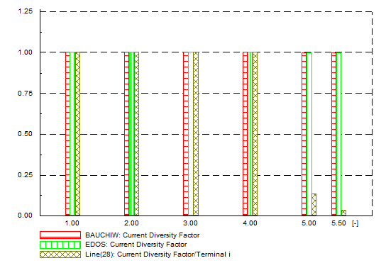 | Figure 19. Balanced network - current diversity factor |
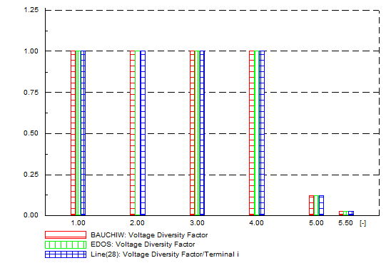 | Figure 20. Balanced network - voltage diversity factor |
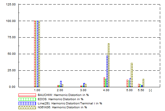 | Figure 21. Unbalanced network - harmonic distortion |
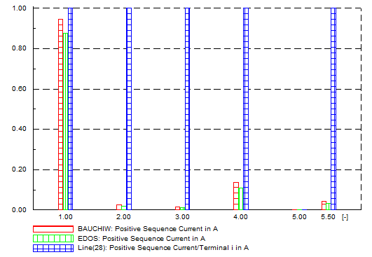 | Figure 22. Unbalanced network-positive-sequence current, A |
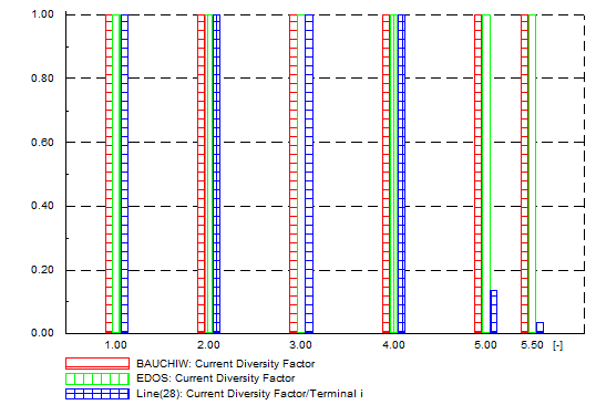 | Figure 23. Unbalanced network - current diversity factor |
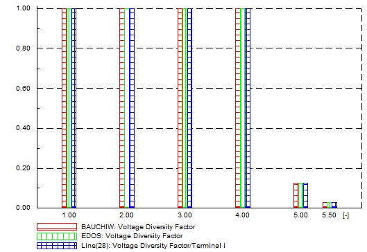 | Figure 24. Unbalanced network - voltage diversity factor |
 | Figure 25. Frequency sweep - current diversity factor |
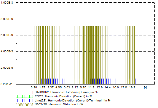 | Figure 26. Frequency sweep - harmonic distortion (current) |
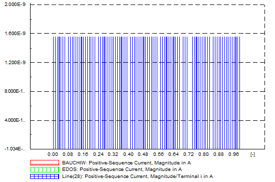 | Figure 27. Frequency sweep - positive-sequence current |
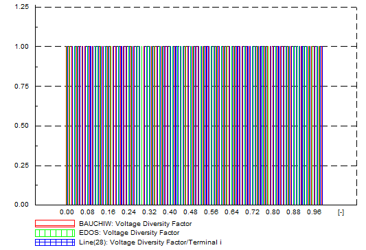 | Figure 28. Frequency sweep - voltage diversity factor |
10. Conclusions
- Basic analyses were carried out in this paper (part I) and includes load flow, short-circuit calculation, transient stability, modal analysis/eigenvalues calculation and harmonics analysis. Short-circuit analysis is used in determining the expected maximum currents (for the correct sizing of components) and the minimum currents (to design the protection scheme), while transients, stability analyses important considerations during the planning, design and operation of modern power systems. One common application of harmonic analysis is providing solution to series resonance problems.
APPENDIX
- Nomenclature
 peak current;
 breaking current (RMS value);
 peak short-circuit breaking current;
 initial symmetrical short-circuit current;
 peak breaking apparent power;
 decaying d.c. component;
 thermal current;
 load current;
 initial short-circuit current;
 factor for the calculation of
  ;
; factor for the heat effect of the d.c. component
 factor for the heat effect of the a.c. component;
  are nominal conditions.
 generator speed vector
 ith eigenvalue
 ith right eigenvector
 magnitude of excitation of the ith mode (at t=0);n number of conjugate complex eigenvalues PARAMETERS USED FOR POWERFACTORY ANALYSIS(ⅰ) Wind generator data (output = 50 MW):Static generator (wind) ratings = 3MVA; active power = 2MW; power factor = 0.95; terminal voltage = 0.69kV; number of generators = 25; (ⅱ) Solar generator data (output = 50 MW):Static generator (solar) ratings = 0.6MVA; active power = 0.5MW; power factor = 0.95; terminal voltage = 0.4kV; number of generators = 100; (ⅲ) Synchronous generator controllers data:• PSS:
 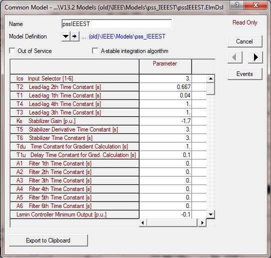 • AVR:
 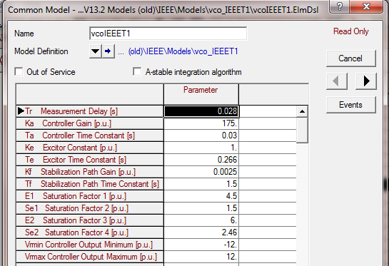 • Turbine and governor:
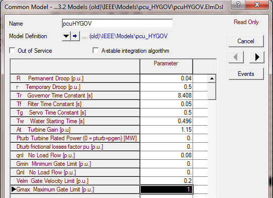
References
| [1] | Sambo A. S., Garba B., I. H. Zarma and M. M. Gaji, “Electricity Generation and the Present Challenges in the Nigerian Power Sector”, Unpublished Paper, Energy Commission of Nigeria, Abuja-Nigeria, 2010. |
| [2] | www.google.com/publicdata. |
| [3] | ThisDay Newspaper, 3rd October, 2011. |
| [4] | www.energy.gov.ng. |
| [5] | Magazine article; African Business, No. 323, August-September 2006. |
| [6] | Ileoje, O.C., “Potentials for Renewable Energy Application in Nigeria, Energy Commission of Nigeria”, pp 5-16, 1997. |
| [7] | Fagbenle R.L., T.G. Karayiannis, “On the wind energy resource of Nigeria”, International Journal of Energy Research. Number 18, pp 493-508, 1994. |
| [8] | Okoro, O.I. and Madueme, T.C.: “Solar energy investments in a developing economy”,Renewable Energy 29, 2004, pp. 1599-1610. |
| [9] | Garba,B and Bashir, A. M (2002). Managing Energy Resources in Nigeria: Studies on Energy Consumption Pattern in Selected Areas in Sokoto State. Nigerian Journal of Renewable Energy, Vol. 10 Nos. 1&2, pp. 97-107. |
| [10] | M. S. Adaramola and O. M. Oyewola, ‘Wind Speed Distribution and Characteristics in Nigeria’, ARPN Journal of Engineering and Applied Sciences, VOL. 6, NO. 2, FEBRUARY 2011. |
| [11] | Gonzalez-Longatt F.M., ‘Impact of Distributed generation over Power Losses on Distributed System’, 9th International Conference, Electrical Power Quality and Utilization, Barcelona, 9-11 October, 2007. |
| [12] | M. Begović, A. Pregelj, A. Rohatgi, ‘Impact of Renewable Distributed Generation on Power Systems’, Proceedings of the 34th Hawaii International Conference on System Sciences, 2001. |
| [13] | Mohamed El Chehaly ‘Power System Stability Analysis with a High Penetration of Distributed Generation’, Unpublished M.Sc. Thesis, McGill University, Montréal, Québec, Canada, February 2010. |
| [14] | DIgSILENT PowerFactory Version 14.1 Tutorial, DIgSILENT GmbH Heinrich-Hertz-StraBe 9, 72810 Gomaringen, Germany, May, 2011. |
| [15] | Saadat H., “Power System Analysis”, McGraw- Hill International Editions, 1999. |
| [16] | http://webstore.iec.ch/preview/info_iec60909-0%7 Bed1.0%7Den_d.pdf |
| [17] | Serrican A.C., Ozdemir A., Kaypmaz A., ‘Short Circuit Analyzes Of Power System of PETKIM Petrochemical Aliaga Complex’, The Online Journal on Electronics and Electrical Engineering (OJEEE), Vol. (2) – No. (4), pp 336-340, Reference Number: W10-0037. |
| [18] | Patel J.S. and Sinha M.N.‘Power System Transient Stability Analysis using ETAP Software’, National Conference on Recent Trends in Engineering & Technology, 13-14 May 2011. |
| [19] | Iyambo P.K., Tzonova R., ‘Transient Stability Analysis of the IEEE 14-Bus Electrical Power System’, IEEE Conf. 2007. |
| [20] | Dashti R. and Ranjbar B, ‘Transient Analysis of Induction Generator Jointed to Network at Balanced and Unbalanced Short Circuit Faults’, ARPN Journal of Engineering and Applied Sciences, Vol. 3, No. 3, June 2008. |
| [21] | Kundur P. ‘Power System Stability and Contrl’, The EPRI Power System Engineering Series, McGraw-Hill, 1994. |
| [22] | Kumar G.N., Kalavathi M.S. and Reddy B.R. Eigen Value Techniques for Small Signal Stability Analysis in Power System Stability’, Journal of Theoretical and Applied Information Technology, 2005 – 2009. |
| [23] | IEEE Recommended Practices and Requirements for Harmonic Control in Electrical Power Systems, IEEE Std. 519-1992, 1993. |
| [24] | Manmek T., Grantham C. and Phung T. ‘A Real Time Power Harmonics Measuring Technique under Noisy Conditions’, Australasian Universities Power Engineering Conference, Brisbane, Australia, 26th-29th September 2004 |