David Becerra, Jorge Ortiz, Zoila Ramos
Department of ComputerSystem and Industrial Engineering, Universidad Nacional de Colombia, Bogota, Colombia
Correspondence to: David Becerra, Department of ComputerSystem and Industrial Engineering, Universidad Nacional de Colombia, Bogota, Colombia.
| Email: |  |
Copyright © 2012 Scientific & Academic Publishing. All Rights Reserved.
Abstract
Using power lines to transmit telecommunications has become one of most suitable options to offer tele-communications services over IP protocol, due to an economic benefit that comes from utilizing a preexisting infrastructure. However, electric grid wasn’t made for telecommunications purposes, causing several undesired effects such as: multipath behavior similar to wireless network without fast fading, electromagnetic interference, different sources of noise and change of channel’s response due to loads connected to the grid. This paper shows what kinds of variations of response exist and how this effects can be treated using a stochastic modification of Zimmerman’s model of PLT network.
Keywords:
PLT, PLC, BPL, Stochastic Channel Response, Loads Effects
Cite this paper:
David Becerra, Jorge Ortiz, Zoila Ramos, "Stochastic Behavior of Electric Grid Channel for Power Lines Telecommunications Due to Loads on In-Home Environments", Electrical and Electronic Engineering, Vol. 2 No. 6, 2012, pp. 379-382. doi: 10.5923/j.eee.20120206.06.
1. Introduction
Power line telecommunications, also known as broadband powerline or power line communications (PLT, BPL and PLC), is defined as the usage of electric infrastructure to provide telecommunications services, option that brings several benefits to users and service providers as no need of building a new infrastructure what is appreciate in terms of cost, hence there is no necessity of make modifications on buildings causing an enormous interest to many actors in telecommunication’s sector including normalizations organism. Nonetheless, electric wire’s characteristics are not the best for transmitting telecommunications signals; this network was originally intended to carry just electrical energy making this medium hostile to high frequency signals.As an emergent and important technology, PLT needs a model that represents its main qualities for implementation purposes, however most models are deterministic causing troubles when is necessary to apply them in other scenarios with different conditions. The Institute of Electrical and Electronics Engineers (IEEE) has taken this necessity into account, and has chosen a model that can accomplish these requirements[1], nonetheless there are some qualities that are out of model’s scope, like loads effects over channel response, in fact ignoring this effects can cause a decrease on performance of 60% for broadband communications[2].This paper pretends to show how effects due to change of loads on a network in-home can be added to the model chosen by IEEE using statistics theory. First, we are going to do a review about channel model. Second, a classification of loads behavior and how they can be modeled is shown. Third, a way to add this behavior to model will be explained and last conclusions are presented.
2. PLT Channel Review
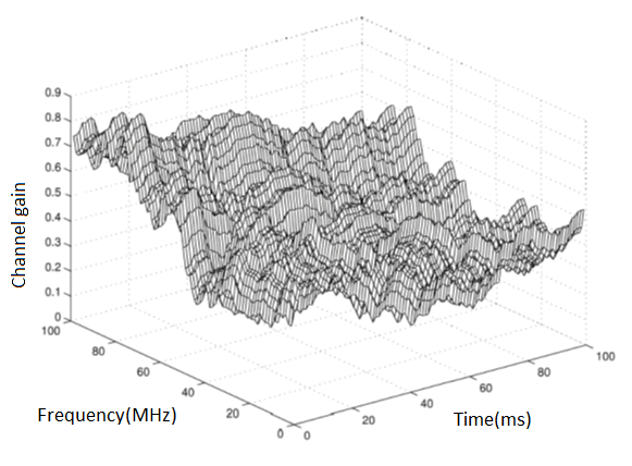 | Figure 1. 3D representation of channel response |
Due to the importance of PLT in telecommunication’s sector two of the most avowed organism, IEEE and International Telecommunication Union (ITU), have been working on standardization of this technology, generating two standards, IEEE 1901 and ITU Ghn 9960 with different scopes and environments to apply. Additionally, IEEE generated a document where they select a channel model to make easier implementing this technology from all existing until September 2010[]; this model have to be stochastic because of channel’s response change with time and frequency, it can be seen as a random variable indexed in time and frequency, this is showed inFigure 1.The IEEE made an extensive research between PLT models available and chose Zimmerman’s model[] because it represents multipath effect with a maximum of physical phenomena even being a top-down approach. Besides a probability density function can be defined easily. The mathematical form of this model is expressed on equation (1).This model uses the sum of every possible way’s transfer function that a signal can found between the transmitter and the receiver. These functions are obtained applying transmission line theory to PLT network, using Distributed parameters, which are depicted inFigure2; everyone represents a lumped abstraction per unit of length that can be found using electromagnetic theory to the geometric configuration of conductors. | (1) |
Weighting factor give a measure of how much is i-th path contributing to total result and is calculated by multiplying all reflection and transfer coefficients on the way; attenuation express the dependence of gain regard frequency and distance; meanwhile delay defines the retardation of signal when it takes the path i.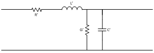 | Figure 2. Distributed parameters |
2.1. Calculation of Factors
Zimmerman model has two types of factors, ones which depends on path like weighting and delay, and attenuation that is general for all trajectories. First, attenuation is computed using the propagation constant when transmission line is matched, which is defined in (2). Hence transfer function can be expressed in terms of its length(3). | (2) |
 | (3) |
Due to frequency range where PLT works, γ can be simplified because of  and
and , result showed in (4), where ZL is the characteristic impedance of the transmission line, defined in (5).
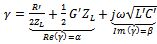 | (4) |
 | (5) |
Resistance of conductors may be proportional to square root of frequency or frequency itself. Meanwhile, losses due to dielectric presence are directly proportional to f. This is demonstrated using equations to obtain R and G on 2 parallel conductors of radius r.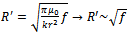 | (6) |
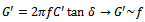 | (7) |
Simplifying, attenuation is bounded to alpha term of gamma, and can be expressed as a function of three constants a0, a1 and k; equations (8) and (9). These parameters can be found using measurements or theoretical calculations. | (8) |
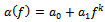 | (9) |
Weighting and delay are obtained from topology of electric grid, in Figure 3 a network composed by a line with one branch is shown, this will be used to make an example of how this parameters are calculated.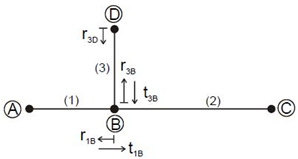 | Figure 3. Grid with one branch connected to main line[1] |
First step is identifying possible paths that a signal can take, the direct path is ABC, however segments of lineare notmatched causing reflections, and hence other option may be ABDBC or ABABC, even ABDBDBC. Every possible path should be consider, however that is unpractical, a criteria must be applied in order to obtain an efficient representation of PLT channel, for example if direct path has a weighting factor of 0.8, channels with this factor above of 0.08 have to be taking into account.After trajectories are defined, a product between reflection and transfer factor of each segment of line is needy to get weighting. Assuming A and C matched (there is no reflection, hence transmission’s value is one) weighting for ABC would be t1b, on ABDBC case it will be t1b*r3d*t3b. Similar process is done to obtain total length for delay and attenuation.Delay factor is dependent of path’s length, using equation (10) these magnitudes are related with dielectric constant of material and light speed.  | (10) |
3. Load’s Behaviorand Classification
In-home environments are different to other sections of electric grid such as house’s exterior low tension network, used as access networkfor PLT communications, or medium voltage, bearer service network in terms of loads behavior. Because Human activities modify network when a device is plugged, turned on, turned off or disconnected, this process cannot be modeled by deterministic methods to implementation purposes. First, human activities is seen by PLT signal as a long term variation, because when a device is plugged the change is “permanent” respect to bit rate. In order to represent this behavior a markov process can be used, and states of system are generalized to two states (ON and OFF)[4] , however there are some devices which influences network when are plugged but off, causing 3 states[5].Additionally, devices must be classified using their behavior when they are connected and on, there are three types. First we have constantimpedances, which are not common and their reasonable values are 5, 50,150, 1000 and infinite, to represent low, RF standard, similar to transmissionline, high, and open circuit respectively[6]; second,time-invariant but frequency-selectiveimpedances like RLC circuits; and last time-varying and frequencyselective, such as devices which use rectifiers with diodes or controlled silicon elements (SCRs or mosfets)[7][8].In[6] these three groups are studied, and for second type an equation is presented (11), impedance is expressed in 3 parameters: R, resistance at resonance;  , resonance angular frequency; and Q, quality factor that is related to bandwidth.
 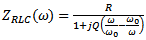 | (11) |
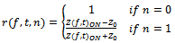
Third group can be divided in two subgroups: one is related to devices that works commuting between two states, therefore this group have two values associated and are synchronous to period of electric energy signal, in order to simplify calculates transition between two states can be ignored for rectifiers with diodes because of short time of one state compared with period of main; the other one correspond to an harmonic variation along mains voltage that is modeled in (12), where ZA is the impedance that is presented all time as an offset, ZB represents the amplitude of harmonic variation and θ refers to difference with zero cross of main voltage. Devices in last group are commonly small appliances. | (12) |
4. Stochastic Zimmerman Addition
Due to Zimmerman’s model composition is clearly that loads affects the weighting factor because of reflection and transmission coefficients definition on equations (13) and (14). | (13) |
 | (14) |
If ZL was a constant time invariant weighting factor would be constant too for every possible path. However, this isn’t the case and transfer function has to be redefined using equation(15). Hence, weighting factor can be defined as a function dependent on set of j random variables and each variable is a reflection coefficient due to a load, impedance is not used because the relation between reflection coefficient and weighting factor is simpler than impedance’s relation, this is important if a probability density function is needed and is obtained by transformations.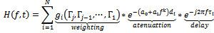 | (15) |
Some assumptions have to be done in order to obtain a good addition of stochastic effects: First, there are two kinds of reflection coefficients, those due to loads and constant ones, this are caused by connections between cables. Each load only can cause a reflection coefficient, and then each load’s node, point where a load is plugged, must be connected only with one node, an example of topologyis shown on Figure 4 where Z1, Z2 and Z3 are common loads while ZG and ZL are impedances of PLT devices.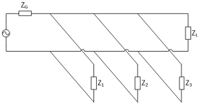 | Figure 4. Topology with one connection per load |
Second, all random variables are independent or uncorrelated; it means that a state (on or off) of a load doesn’t depend on other states of the rest of charges plugged to the electric grid.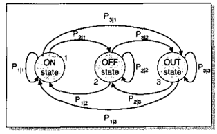 | Figure 5. state diagram of the loads |
With assumptions made, defining reflection coefficient variable is the next step. These random variables are modeled with a markov process using two or three states as load requires depicted in Figure 5, where value of reflection on each estate is defined by load type and times of states are exponential distributed. Commonly only two states are used, most people doesn’t plug off their devices when are off, on and off then states can be defined as Figure 6, 0 when device is off and 1 for on. Hence, Reflection would be defined as function of frequency, state n and time (depending on type of load), shown on equation (16).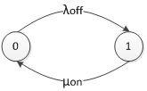 | Figure 6. State diagram |
 | (16) |
This is a truncated Poisson distribution with n=1, then reflection factor has two possible values and a probability associated, which is shown on equation (17), is necessary to obtain average times of use in order to get probabilities for each state. 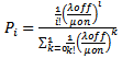 | (17) |
Then the joint probability mass function is constructed by the multiply of each reflection coefficient’s distribution function (18).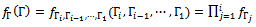 | (18) |
Now is possible to calculate expected value of channel response (an important value to take into account when a system is designed),it depends on weighting factor because attenuation and delay aren’t determined by loads and are constants to each path (distance doesn’t change). As linear operator, expected value of Zimmerman’s model would be expressed in equation(19), where att and de refers to attenuation and delay. | (19) |
 | (20) |
In equation (20)this problem is reduced to find the expected value of weighting factor, which was defined as a function. Then the definition of expected value of a function is applied on (21). | (21) |
5. Conclusions
There is no independence between transmission and reflection factors due to same load and because of that, is better to applied expected value to weighting factor as a function. By the other hand, joint probability function can be obtained using transformations of variable set for designing or implementing purposes.If there is a need, the process explained here can be extended to devices with three states of behavior and load’s function for third state must be known.Time series of this model can be generated for simulation purposes and it’s possible to use period of main voltage to replace time index due to periodicity of loads.Knowledge about topology is needed, specifically distances, characteristic impedance of every segment (it can be related to diameter) and loadsplugged on electric grid in order to use this addition, data can proceed of theory calculations or measurements.Channel responsecould be used to improve broadband communications over power line either telecommunication services or smart grids applications on in-home environments, for example a set of desirable frequencies can be selected for transmitting with low bit error rate while others frequencies are neglected when a system is being designed or implemented. Hence, using expected value of channel response a set of frequencies can be selected in order to obtain an optimal transmission.
References
| [1] | IEEE 1901 working group. (2012, Sep) Electrical Network and Topology. |
| [2] | Avril G, Etude et Optimisation des Systèmes à Courants Porteurs, 2008, thesis of "Institut National des Sciences Appliquées de Rennes, France". |
| [3] | K.Dostert M. Zimmermann, "A Multi-Path Model for the Power Line Channel," IEEE Transactions on communications, vol. 50, no. 4, pp. 553-559, april 2002. |
| [4] | S. Sancha, F.J. Canete, L. Diez, and J.T. Entrambasaguas, "A Channel Simulator for Indoor Power-line Communications," in Power Line Communications and Its Applications, 2007, pp. 104-109. |
| [5] | F.J. and Diez, L. and Cortes, J.A. and Entrambasaguas, J.T. Canete, "Broadband modelling of indoor power-line channels," Consumer Electronics, IEEE Transactions on, vol. 48, no. 1, pp. 175 -183, feb 2002. |
| [6] | F.J. and Corté ands, J.A. and Dí andez, L. and Entrambasaguas, J.T. Canete, "A channel model proposal for indoor power line communications," Communications Magazine, IEEE, vol. 49, no. 12, pp. 166 -174, december 2011. |
| [7] | K.J. Jian Sun and Karimi, "Small-signal input impedance modeling of line-frequency rectifiers," Aerospace and Electronic Systems, IEEE Transactions on, vol. 44, no. 4, pp. 1489 -1497, oct 2008. |
| [8] | Sarah Rönnberg. (2011) Power Line Communication and Customer Equipment. [Online]. www.ltu.se |
 Abstract
 Reference
 Full-Text PDF
 Full-Text HTML