Janusz Gajda , Tadeusz Sidor
Chair of Metrology and Electronics, AGH-University of Science and Technology, Krakow, 30-059, Poland
Correspondence to: Tadeusz Sidor , Chair of Metrology and Electronics, AGH-University of Science and Technology, Krakow, 30-059, Poland.
| Email: |  |
Copyright © 2012 Scientific & Academic Publishing. All Rights Reserved.
Abstract
Sensitivity of electronic circuits to component tolerances has been the topic of many papers[5],[6],[9], discussing sensitivity analysis tools, but seldom they give advices how without many preparations perform practical analysis of a circuit which is not provided for mass-production. And this is often the case in the field of measuring transducers, which sometimes are design to be used in one unique application in various fields of research. This paper presents practical employment of the Monte Carlo analysis to compare sensitivity of different structures of electronic converters to component tolerances. The method enables to determine limiting error of the structures and to point out the structure, which is less sensitive to component tolerances. Although the way the Monte Carlo analysis has been used is far from optimal and requires redundant simulations it can be employed strait away at any stage of the converter designing process without being involved in complicated calculations, or additional programming. It uses ready made, commercially available software built in most of circuit analysis programs. E.g. the working demo version of MICROCAP, which is free for students and university staff, has been used in this case. Although the demo version has limits in its applications, is usually sufficient for most of the cases.
Keywords:
Monte Carlo Analysis, Component Tolerances, Simulation
Cite this paper:
Janusz Gajda , Tadeusz Sidor , "Using Monte Carlo Analysis for Practical Investigation of Sensitivity of Electronic Converters in Respect to Component Tolerances", Electrical and Electronic Engineering, Vol. 2 No. 5, 2012, pp. 297-302. doi: 10.5923/j.eee.20120205.09.
1. Introduction
All electronic circuits performance depend on the values of their component parts, and the values can never be exactly known, as all of them have specified tolerances. The influence of each component value on the circuit performance can be very significant or vice versa. It can be described by defining circuit sensitivity to the variation of each of the component value. Relative sensitivity  than can be defined as partial derivative of the chosen circuit response y in respect to the given component value x variations.
 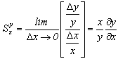 Even if all circuit sensitivities are known it is not enough to evaluate limits of circuit response, as the exact differences of component values from their nominal values are not known. There are few different approaches, if the yield of circuits provided for mass production is to be evaluated. Most of them require prior calculation of circuit sensitivities. One of the method uses adjoined network to calculate sensitivities, the other expansion of circuit transfer function into Taylor series and taking only derivatives of first order into account, or approximate derivatives by using finite increments of circuit parameters value[5],[6],[7],[8],[9]. When circuit sensitivities are found than EVA (Extreme Value Analysis) or an RSS (Root Sum Squared) approach is used[7],[14] to evaluate the worst-case tolerance limits for the circuit. The alternative approach is to use Monte Carlo analysis, which does not require circuit sensitivity calculation, but by multiple repetition of simulated circuit performance with randomly varied component values can give estimation of circuit performance limits[6],[10],[11],[15].All of the methods require a lot of computation and access to specific software, and this can be a real problem in case of analysis in designing process of measuring transducers, which sometimes are intended to be used in one unique application in various fields of research. It would not be economical to spend too much time to develop any special method for such analysis.In reality the design is usually entirely based on designer experience and its usefulness is later verified by experiments.The Monte Carlo analysis feature, which is built in the most of the circuit analysis programs, seems to be reasonable solution to help designer of electronic transducer, at least, to select most promising circuit structure, when its sensitivity to components tolerances is taken into consideration. The other approaches are far too laborious to be used, as even to formulate the conversion function of the circuit is quite a tedious task, and evaluate expression of total derivative is prohibitively complicated. It can be seen in the case of very simple circuits, analysis of which are presented e.g. in[5],[9],[15].The Monte Carlo analysis, as such, can be performed assuming various distributions of component values within the specified tolerance. The Gaussian distribution is seldom used, as taking into account the component selection method used by manufacturers the uniform distribution is rather to be expected[12]. In case of electronic instrumentation converters it is important to evaluate their limiting error value and for such a task the Worst Case Monte Carlo analysis should be chosen. It means that in each simulation all the components parameter values are chosen randomly, but only as border values from the tolerance range.The limiting error values can be further used as a criterion e.g. to compare and point out the circuit structure, which is less sensitive to component tolerances.Values of the component parameters can only be obtained within certain tolerance, which affect the converter precision i.e. causing certain error. This kind of error, further named as the structure error, depends on values of the components tolerances as well as the instrumentation converters structure. Many electronic instrumentation converters, to perform a given measuring task, can be built using different principle of operation i.e. using different circuit structures and different components. Usually the value of component parameters has to be chosen very precisely because it determines accuracy of operation of the electronic transducer. The same device, for instance the instrumentation amplifier, can be built in two different ways. The question is, if it is possible to select structure, which is less sensitive to component tolerances, and therefore is more suitable for given measurement application. In this paper the linear rectifier circuit and the instrumentation amplifier circuit have been compared as examples to show how the Monte Carlo analysis can be employed to find out the structure of electronic circuit, which is more suitable to be used as instrumentation transducer. The Monte Carlo analysis offered by circuit analysis programs MICROCAP[4] has been used for it.
2. Using the Monte Carlo method
Monte Carlo analysis bases on multiple, but limited in number, runs of circuit performance simulation with different set of circuit components values each time. So, the question arises if in the amount of scheduled runs the set of randomly chosen component values would include the case, which determines the highest value of the structure limiting error. When number of simulations increases the probability of an event that the worst combination is taken into account rises. To determine probability of that event Bernoulli theorem can be used.When an electronic device or instrumentation converter consists of L components of given tolerances and the each component parameter value can take only the "border value" (maximum or minimum) it means that only N = 2L possible values have to be taken into account. Probability p of an event that one of N configurations exists in one simulation is equal p=1/N. Probability that in K attempts (K >> N) at least one chosen configuration of elements values can be found, is given by (1):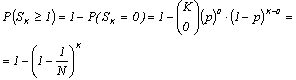 | (1) |
where: SK - number of how many times in K simulations the worst-case parameters configuration is detectedProbability that in K trials all the component values are taken into account is the N power of single component combination probability according to (2): 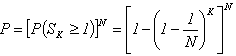 | (2) |
In the case of only few components the required number of simulation runs, which secure ninety percent probability level that the worst case was found is given in Table 1.| Table 1. Number of Simulation Runs, which Secure Ninety-percent Probability Level |
| | Number of components | Number ofconfigurations | Number of simulationsruns (P>90%) | | 4 | 16 | 78 | | 5 | 32 | 180 | | 6 | 64 | 407 | | 7 | 128 | 906 |
|
|
Using formula (2) to determine the required number of simulation runs to achieve reasonable confidence level it can be seen that the number rises very quickly with the number of parameters subject to random variations.There are mathematical methods[11] which when used to control the process of random variation can significantly reduce the required number of runs if only the percentage yield of circuits provided for mass production is relevant.This is not the usual situation in the case of instrumentation transducers where the worst-case performance of circuits is of prime importance and the tools for such analysis should be as simple as possible.This is why it is more practical to use Monte Carlo package, as it is, available in the circuit analysis program to run simulation e.g. 906 times in the case of 7 varying elements instead of developing special software which could cover all possible elements combination in only 128 runs.
3. Examples
3.1. Comparing Sensitivity to Component Tolerances of Two Different Structures of Linear Rectifiers
To measure accurately half period mean value of sine-wave type signal of small magnitude it is necessary to employ rectification method that can eliminate the threshold voltage of ordinary diodes. The circuits named linear rectifiers are commonly used in such case. There are at least two different structures of linear rectifiers, which can be found in literature. They are shown in the figure la and 1b respectively.Resistor values of the linear rectifier shown in the figure la have to be selected according to the following[2],[3]: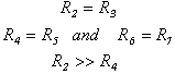 For the correct operation of the linear rectifier structure in the figure l b the following conditions have to be met:
 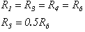 To find out which of these two structures is less sensitive to tolerances of passive components used to assembly the structure, the Monte Carlo analysis of the Micro Cap software was used. Simulation was carried out in the time domain. As an input sinusoidal signal source was used. The mean value of the output signal was assumed to be the output of the structure.
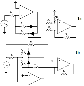 | Figure 1. Two equivalent structures of linear rectifier |
As the question was to find out how the resistor tolerances influence the performance of the circuits, to eliminate the possible influence of operational amplifiers parameters they were replaced by the ideal models i.e. depended voltage sources of very high, independent of frequency gain, equal to 1015[V/V]. Resistors tolerance was chosen equal to 1%. To compare these two structures the following definition of the conversion error was chosen (8).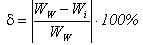 | (3) |
Where Wi is the half-period mean value of the rectified signal obtained during the simulation for one of the component value combination. WW is the theoretical half period mean value of the sinusoidal input signal equal to: Rectifier shown in figure la contains six passive elements. If each resistor can randomly assume one of the extreme values from the tolerance range, it means that sixty-four possible combinations of component values exist. It determines the number of simulations required producing all of the combinations including the worst one. In this case 407 simulations have to be made to secure 90 % confidence level according to equation (2).Rectifier shown in figure 1b is assembled with seven passive elements. In this case to secure the same confidence level 906 simulations have to be carried out.
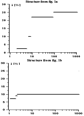 | Figure 2. Limiting error value as function of numbers of simulation runs |
Results of those simulations are shown in figure 2. On the Y-axis the limiting (8) error value is shown, as the function of the number of simulations (N). After certain number of simulations the error value reaches practically constant level, which can be considered as a proof that all (including the worst one) passive elements combinations have been used.Limiting error value for the structure in figure la is estimated as 25.12% (for assumed 1% resistor tolerances) and for the structure in figure 1b is equal 10.84%. So, it is possible to state that the structure shown in figure 1b is less sensitive to resistor tolerances, although to obtain sensible level of limiting error the resistors of much smaller tolerances should be used.
3.2 Comparing Parameters of Two Different Structures of Instrumentation Amplifiers Sensitivity to Component Tolerances
Instrumentation amplifiers can also be built in different configurations. Two possible different structures are shown in figure 3a and 3b respectively. As only sensitivity of the structures parameters to passive element tolerances is investigated, as previously the ideal models of OpAmps have been used.The differential gain of the structure in figure 3a is given by formula (4),[1],[3],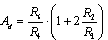 | (4) |
if the following conditions are fulfilled:R2 = R3 ; R5 · R6 = R4 · R7The resistor R1 value sets the amplifier gain.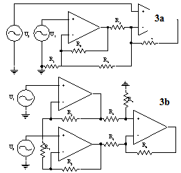 | Figure 3. Two different structures of instrumentation amplifiers |
The differential gain of the amplifier for the structure shown in fig figure 3b is given by (5). 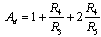 | (5) |
R2 · R4 = R1 · R3 The R5 resistor value sets the amplifier gain.One of the most important features of any instrumentation amplifier is its ability to reject common input signal (CMRR). The Monte Carlo method has been used, in the similar way as for the linear rectifiers, to compare the sensitivity of CMRR of both structures to resistor tolerances. As previously, the number of simulations runs was set according to the number of resistors in the structure (Table 1).For the amplifier structure in figure 3a, which is built of six resistors, more than 407 simulations have to be performed. For the structure shown in figure 3b, built of four resistors only, 78 simulations have to be carried out to achieve the same probability confidence level.For the simulations the AC analysis of the Micro Cap have been used. Simulations were performed for different values of the amplifiers differential gain (Ad). CMRR values for both structures have been calculated as the ratio of the differential gain to the highest common gain value. To calculate the differential gain value for the both structures the equations (4) and (5) was used respectively.Results of the simulations are shown in figure 4 as the relation between the CMRR and differential gain Ad. From the graph it is possible to state that the CMRR of the two Opamp structure (figure 3b) is less sensitive to resistor tolerances.Another important feature of any instrumentation amplifier is its differential gain value. To study how the differential gain of both amplifier structures depends on resistor tolerances again the Monte Carlo analysis of the Micro Cap have been used.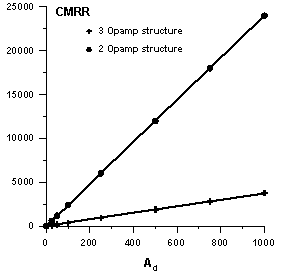 | Figure 4. The smallest values of CMRR for two different structures of instrumentation amplifiers |
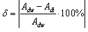 | (6) |
The largest value of δi can be interpreted as absolute limiting error of the gain for the given structure. The relation between the relative error value of differential gain and the theoretical differential gain value is shown in the figure 5.From the graphs it is possible to state that the differential gain of the structure built of two OPAMPS (figure 3b) is more immune to resistor tolerances than the structure of three OPAMPS (figure 3a) for differential gain values smaller then 10[V/V]. For the differential gain values greater than 10, the structure built of three OPAMPS is less sensitive to the resistor tolerances. | Figure 5. Limiting error of differential gain |
4. Conclusions
Presented method can be very useful when designing a circuit e.g. electronic transducer, which sometimes is provided to be used in one unique application, and is not provided for mass-production. In such situation it would not be economic to get involved in complicated calculations, or additional programming, which certainly can lead to more efficient method of sensitivity analysis.In the paper we present the application of the method to compare different structures of circuits, which can perform similar operation, and the results can be used to select which of the structures is less sensitive to the component tolerances i.e. is more suitable to be used as measuring transducer. The method requires specification of a criterion to evaluate the performance of the compared structures.It has to be kept in mind that in Monte Carlo analysis the combinations of component values are chosen in a random way. To say that one of the structures is less sensitive than another, simulations have to be carried out many times, to secure that all of the component tolerance combinations, including the worst one, have been found. Whether all of the components tolerances combinations were simulated can be assumed only with certain probability, which can be high (equation (2)) if sufficient number of simulations is performed. The time required to perform the sufficient number of simulations depends on the type of the circuit and required number of simulations.As an example of practical employment of the method comparative sensitivity analysis of two possible structures of linear rectifier has been presented. The results make possible to state that the structure shown in figure 1b is less sensitive to component tolerances, and therefore more suitable to be used as measuring converter.Another example, concerning instrumentation amplifier performance, shows that the structure presented in figure 3b is less sensitive to resistor tolerances when CMRR, and differential gain, larger than ten, is taken into account. For smaller differential gains, its value seems to be less sensitive for the structure presented in figure 3a. From our experience we can say that the total simulation time never exceeds a few hours, for each circuit, even when more then 500 simulations runs have been performed. Moreover, many simulations, which were carried out, proved that realization of as many simulations as equation (2) requires for 90% probability confidence level is usually sufficient.
References
| [1] | Charles Kitchin, Lew Counts, “A designer's guide to instrumentation amplifiers”, Analog Devices, Inc. 2000. |
| [2] | Daniel H. Sheingold, “Nonlinear circuits handbook” ,Analog Devices, Inc. Norwood, Massachusetts 02062 U.S.A., 1976. |
| [3] | Ulrich Tietxe, Christof Schenk, „Halbleiter Schaltungstechnik“, Springer-Yerlag Berlin Heidelberg, 1993. |
| [4] | Spectrum Software: Micro-Cap Electronic Circuits Analysis Program. Reference Manual 1999. |
| [5] | Mark Fortunato (2008) “ Analysing circuit sensitivity for analog circuit design”, EE/Times Design 4/16/2008 |
| [6] | Cesare Alippi, Marcantonio Catelani, Ada Furt, Marco Mugnaini , “ SBF Soft Fault Diagnosis in Analog Electronic Circuits: A Sensitivity-Based Approach by Randomized Algorithms” IEEE Trans. On Instrumentation and measurements. Vol. 51, No 5, Oct 2002 |
| [7] | “Design and analysis of Electronic Circuits for Worst Case Enviroments and Part variations”, NASA Preferred Reliability Practices No PD-ED 1212 |
| [8] | Denis Duret, Laurent Gerbaut, Frederic Wurtz, Jean-Pierre Keradec, Bruno Cogitore, “ Modelling of passive electronic circuits with sensitivity analysis dedicated to the sizing by optimization”, Proceedings KES’07/WIRN’07, Springer Verlag 2007 |
| [9] | E.A. Gonzalez, M.C.G. Leonor, L.U. Ambata, C.S. Francisco, “Analysing Sensitivity in Electronic Circuits”, IEEE Multidiciplinary Engineering Education Magazine Vol. 2, No1, March 2007 |
| [10] | W.M. Smith, “Worst-Case Circuit Analysis for Electronic Parts “, MEDICAL ELECTRONIC design Sept. 1999. |
| [11] | Robert Spence, Randeep Singh Soin, “ Tolerance Design of Electronic Circuits”, Imperial College Press 1977. |
| [12] | Ray Kendall, “Worst Case Analysis Method for Electronic Circuis and Systems to Reduce Technical Risk and Improve System Reliability”, Intuitive Research and Technology Corporation. Apr. 2007. |
| [13] | Robert Boyd, “Tolerance Analysis of Electronic Circuits Using MATHCAD”, CRC Press Sept. 1999. |
| [14] | Steven M. Sandler, “A Comparison of Tolerance Analysis Methods”, (1998) AEi Systems, LLC. Online Available: www.ema-eda.com |
| [15] | Andrew G. Bell, “Risk Assesment of a LM 117 Voltage Regulator Circuit Design Using Crystal Ball and Minitab”, (2006) Online Available: www.robustdesignconcepts.com |
 Abstract
 Reference
 Full-Text PDF
 Full-Text HTML