-
Paper Information
- Next Paper
- Previous Paper
- Paper Submission
-
Journal Information
- About This Journal
- Editorial Board
- Current Issue
- Archive
- Author Guidelines
- Contact Us
Electrical and Electronic Engineering
p-ISSN: 2162-9455 e-ISSN: 2162-8459
2012; 2(5): 277-283
doi: 10.5923/j.eee.20120205.06
Linear Invariant Statistics for Signal Parameter Estimation
 Abstract
 Reference
 Full-Text PDF
 Full-Text HTML
Vyacheslav Latyshev
Moscow aviation institute (national research university), department of Radio Electronics aircraft, Moscow, 125993, Russia
Correspondence to: Vyacheslav Latyshev , Moscow aviation institute (national research university), department of Radio Electronics aircraft, Moscow, 125993, Russia.
| Email: |  |
Copyright © 2012 Scientific & Academic Publishing. All Rights Reserved.
This paper presents an approach to obtain an invariant statistics for estimation interested signal parameters independently from unwanted parameters in two dimensional parameter problems. The proposed algorithm is based on the exclusion of Fisher’s information about the unwanted parameters and maintaining information about the parameter of interest. Simultaneous reduction the partial Fisher information matrices to diagonal forms provides the key steps for separation of the signal space into two orthogonal subspaces, containing Fisher’s information about different parameters. The proposed approach requires knowledge of the statistical distributions of signals of interest. The application examples with time delay and Doppler shift as the parameters are provided as a means of evidencing the advantages of the theory.
Keywords: Fisher’s Information Concentration, Independent Time Delay , Doppler Shift Estimations, Invariant Statistics
Cite this paper: Vyacheslav Latyshev , "Linear Invariant Statistics for Signal Parameter Estimation", Electrical and Electronic Engineering, Vol. 2 No. 5, 2012, pp. 277-283. doi: 10.5923/j.eee.20120205.06.
1. Introduction
- In signal processing tasks the available data usually depend on several parameters at the same time. The most common are the time delay, the Doppler shift, the initial phase and amplitude when signal is reflected or transmitted from moving target. Depending on the problem to be solved some of the parameters we are interested in, while others are not significant. For example the signal processing task of a GPS receiver can be divided into two fundamental parts: signal acquisition and signal tracking. Acquisition is by far the more computationally demanding task, requiring a search across a two-dimensional space of unknown time delay and Doppler shift for each GPS satellite to be acquired. Even acquisition task is made there is always same errors in the estimate of Doppler shift and time delay due to coarseness of the grid[1,2].The processing algorithm for these tasks may be simplified if we find statistics, which depends on time delay and is independent of Doppler shift and vice versa. If statistics do not depend on nuisance parameters change, we call them invariant.To determine the position of a signal on the time axis, Doppler shift is not required. The latter can be regarded as unwanted parameter because its changes complicate the processing of the available data[1,2]. If you want to estimate the time delay only, you need statistics invariant to Doppler shift.Conversely, if you need to determine objects’ speed it is important to estimate the Doppler shift. However, in its turn the errors in the estimating of the range can be considered as the unwanted or nuisance parameters. In this case, it is desirable to have an invariant to the time delay estimation errors statistics.Statistics which are independent of the unwanted parameters can be obtained by averaging procedure for conditional probability density of the data over the unwanted parameters, taking into account their a priori distribution[3]. However, firstly the averaging procedure itself requires a large amount of computations. Secondly, the relevant information about a priori distributions of the unwanted parameters is required, but is usually absent. In this paper we propose a method for finding invariant statistics in the two-parameter problems. These statistics can be used to estimate the parameters independently of one another. This method is based on the orthogonal decomposition of the observed data with the concentration of Fisher information in the first terms of the series[4]. Such an orthogonal series can be used to improve the accuracy of maximum likelihood estimates for parameters that are nonlinearly related to the signals[5-7]. Besides the data dimension reduction with the concentration of Fisher information in a small number of members can dramatically reduce the complexity of the Bayesian estimates[8,9]. Sharing the orthogonal decomposition with the concentration of Fisher information about the Doppler shift and time delay provides a means to obtain statistics that depend on one of the parameters, and do not depend on the other. The ideas presented in[10,11] allow to obtain the invariant statistics for independent estimates of the time delay and Doppler shift. A similar approach for the independent estimates of the Doppler shift and the initial phase is presented in[12].This article presents a method for obtaining invariant statistics in the two-parameter problem. These parameters are the time delay and Doppler shift. We then show how to use the singular value decomposition to obtain the required statistics. Next, we illustrate the method on the results of numerical simulations.
2. Theoretical background
- Let
 denote available data column-vector
  , where
  is a parameter of interest and
  is an unwanted parameter. Additive noise vector
  is a zero-mean circular Gaussian with nonsingular covariance matrix
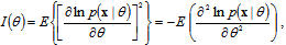
  . First of all, recall that the accuracy of unbiased estimate of an arbitrary parameter
  is determined from the Cramer–Rao inequality (CRI)[3]. In accordance with the CRI the variance is inversely proportional to the Fisher’s information about parameter
  :
: | (1) |
 denotes an expectation,
  - is the conditional probability density function of parameter with known a priori probability density
  . The larger the Fisher’s information the higher the accuracy.The proposed method is based on two facts. Firstly we use an orthogonal decomposition of the observed data with the concentration main part of Fisher information in the first few terms in the series. It allows you to save this information about the estimated parameter in the required statistics. Corresponding theorem proved in[4]. Here it is presented in the appendix. Secondly, if the statistics do not depend on a parameter, it is impossible to estimate it. This statistics don’t contain any Fisher’s information about this parameter and can be considered invariant to its changes. We hope to find the vector of statistics for estimation of
  and at the same time invariant to changes of
  . To obtain it we have to suppress Fisher’s information concerning parameter
  and keep Fisher‘s information concerning parameter
  .Consider
  and
and  , where
  , the superscript H denotes complex conjugate matrix transpose. Matrices
  and
and  can be interpreted as the mean partial Fisher information matrices with respect to
  and
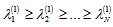
and  correspondingly. In the appendix the eigenvalues and the eigenvectors of an analogous matrix
  in (34) are used to accumulate Fisher’s information in the diagonal elements. Diagonal form of
  reveals actual dimension of the subspace in initial signal space, which contain the most part of Fisher’s information about
  . To provide the invariant to
  statistics we can obtain projection
  onto mentioned subspace and exclude it from
  . The same statement we can conclude concerning
  . On the other hand, the diagonal form of
  reveals actual dimension of the subspace containing Fisher’s information about
  . We have to keep this information because it is connected with accuracy of the
  estimation in accordance with the CRI[3]. To provide both intentions simultaneously let us bring into use next auxiliary matrix
 | (2) |
 | (3) |
 is the identity
  -matrix,
  is the diagonal matrix containing ordered eigenvalues of
  :
:  . Note, that
  provides diagonal form
  too[13]:
 | (4) |
 . It gives the criterion for separation the original signal space into two orthogonal subspaces, containing Fisher’s information about
  and
and  , respectively and exclude Fisher’s information about unwanted parameter. Suppose
  is the actual dimension of subspace, which contains the most part of Fisher’s information about
  . Let
. Let  is a
is a  -matrix, which consists of the first
  rows of
  . Using the linear transformation
  we can obtain invariant statistics for
  estimation. On the other hand the matrix
  is the orthogonal projector onto invariant subspace with respect to parameter
  . Note that, according to[13] (3) can be performed if
  and
and  are chosen to be the matrix of the eigenvalues and eigenvectors of the matrix
  , respectively.Next, we consider this approach on specific examples.
3. Simulation
- Let the N-dimensional data column-vector be an additive mixture of the deterministic component and the distortion vector
 | (5) |
 depends on a priori unknown time delay
  and Doppler shift
  . Assume both parameters are statistically mutually independent. The parameter vector
  has bounded domain of variation, where 2D probability density
  is specified. Let it is necessary to estimate
  from the observation
  only. In this case, the
  can be considered as a nuisance parameter. To find an independent estimate of
  , it is desirable to obtain the statistics in the form of linear functions of vector
  that are not affected by the
  . It is also necessary to minimize possible deterioration of the estimation accuracy, if
  is estimated using these statistics.We use the next two matrices, which are similar to
  and
and  in (2):
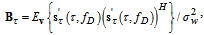 | (6) |
 | (7) |
 and
and  are derivatives. The differentiation are performed with respect to the parameters indicated by the indexes
  or
or  . Symbol
  denotes an expectation over the vector random variable
  .In accordance with (2), let introduce the auxiliary matrix
 | (8) |
 we can divide the observation space into two mutually orthogonal subspaces containing the Fisher information about time delay
  and Doppler shift
  .Finding the matrix C may be complicated if the auxiliary matrix
  is ill-conditioned. In this case we use the following approach. We divide the entire range of the Doppler shift at the L discrete intervals. For each of them we have column vectors
  and
and  , where
  is the middle of the corresponding interval,
  . Let form the following
  matrices:
 | (9) |
 | (10) |
 matrix
  . Then the auxiliary matrix (8) can be obtained as follows
 | (11) |
 we obtain singular value decomposition matrix
  [14]:
[14]: | (12) |
 is
is  diagonal matrix containing the singular values
  of
of  . Matrices
  and
and  are composed of the left and right singular vectors, respectively. For example let
  and the singular values are positive numbers ordered such that
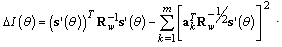
  .From the analysis of singular values we choose the number m to obtain a certain well-defined approximation for
  :
: | (13) |
 and
and  consist of the first
  columns of
  and
and  , corresponding to the largest singular values. If we use the link of the SVD with eigenvalue decompositions[15]:
  | (14) |
 | (15) |
 to
to | (16) |
 gives the orthonormal transformation to diagonalize covariance matrix
  . That is,
 | (17) |
 | (18) |

 and
and  simultaneously. Analysis of the eigenvalues of the matrix
  reveals the dimension of the subspaces containing all or the most part Fisher’s information with respect to the Doppler shift. Suppose it is equal to
 . Then the invariant to the Doppler shift subspace has the dimension
  . Let
. Let  denote the matrix consisting of the first
  columns of
  . Projector onto this subspace:
 | (19) |
 is the dimension of subspaces containing all or the most part Fisher’s information with respect to the time delay. Then the invariant to the time delay subspace has the dimension
  . Let
. Let  denote the matrix consisting of the last
  columns of
  . Projector onto this subspace:
 | (20) |
 | (21) |
 | (22) |
 | (23) |
 is a discrete version of this complex envelope.To illustrate the influence of parameters
  and
and  we can use the Mahalanobis distance between signals[13]:
 | (24) |
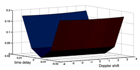
 is the identity matrix, the Mahalanobis distance reduces to the Euclidean distance.Figure 1 shows the Euclidean distance between the delayed signals with the Doppler shift and the signal with zero values of these parameters. The number of samples is fixed to
  , normalized duration of the signal
  . The normalized Doppler shift is the random variable whose behavior is governed by uniform probability density inside a range
  . The relief of the Euclidean distance has a narrow canyon, located at a certain angle to the time axis. Further we consider the time delay as a parameter we are interested in and the Doppler shift as an unwanted parameter.
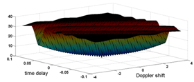 | Figure 1. The Euclidean distance between the chirp signals as a function of the time delay and the Doppler shift |
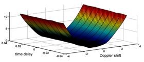
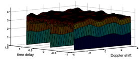
 | (25) |
 and
and  . The approximate matrix (13) has rank
  .
. | Figure 2. The Mahalanobis distance between the projections of the chirp signals onto a subspace invariant to Doppler shift |
 | Figure 3. The Mahalanobis distance between the projections of the chirp signals onto a subspace invariant to small errors in the time delay estimation |
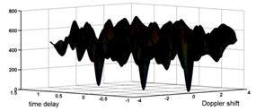
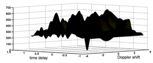 | Figure 4. The Euclidean distance for Gold code of 7 bits |
 are the same as in the previous example. We see here the local gap nearby the true values of
  and
and  . Figure 5 corresponds to the distance (25) for the projections of signals onto the 4-dimensional subspace with the Fisher information concerning
  only. Now the narrow canyon is parallel to frequency axes. It implies that the true value of
  may be estimated independently from
  . The amount of Fisher’s information in the projection onto the specified 4-dimensional subspace is equal to 86% of the amount contained in the observations. Therefore, the estimate of the time delay using the projections is possible with some loss of accuracy.
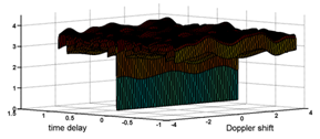 | Figure 5. The Mahalanobis distance between the projections of the Gold code onto a subspace invariant to Doppler shift |
 | Figure 6. The Euclidean distance for the periodic sequences of the Gold |
 | Figure 7. The Mahalanobis distance for the projections of the periodic sequences of the Gold code onto a subspace invariant to Doppler shift |
4. Conclusions
- We have presented the approach to obtain the statistics for signal parameter estimation, which is invariant to unwanted parameter in different two-dimensional parameter problems. The approach is based on excluding Fisher’s information concerning unwanted parameter and saving Fisher‘s information about parameter of interest. The generalized eigenvectors of the matrix pair are used as a means of dividing the observation space into two mutually orthogonal subspaces containing the Fisher information about time delay and Doppler shift. Numerical results show that this approach is effective. To illustrate the procedure the chirp signal and Gold code are used, where time delay is the parameter we are interested in and Doppler shift is the unwanted parameter. The presented approach can be used for estimation problems and for the signal recognition.
Appendix
- Let the observation space corresponds to the set of N observations:
 . Thus, each set can be thought of as a point in a N-dimensional space and can be denoted by a column vector
  , where
  and
and  are the N-dimensional vectors of a signal and a noise correspondingly. Vector
  is Gaussian with nonsingular covariance matrix
  . We assume that
  is known. In general the variable
  appears in a signal in a nonlinear manner. To obtain the m-dimensional vector
  with
with  we use linear transformation
  with the transformation matrix
  . We need such the matrix
  that guarantees minimal losses of estimation accuracy of a parameter
  using vector
  . In addition to foregone requirements we try to represent
  in a new coordinate system in which the components are statistically independent random variables:
  , where
  is a diagonal identity matrix. It is convenient to write transformation matrix in the form of
  . Here
  is a symmetric square root from
  we have
 | (26) |
 in the observation:
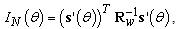 | (27) |
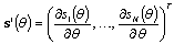 is the column vector of derivatives. The Fisher information in the vector
  [4]:
[4]: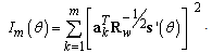 | (28) |
 | (29) |
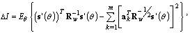 | (30) |
 denotes an expectation over the random variable
  . Thus we need the transformation matrix which provides minimal value of
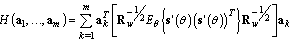
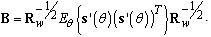
  .Theorem: the linear transformation with the matrix
  provides minimal mean of the loss of the Fisher information
  , if the column vectors
  of
of  are the orthonormal eigenvectors of
 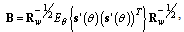 | (31) |
 largest eigenvalues. At the same time
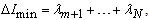 | (32) |
 are the eigenvalues of
  .Proof: let rewrite (30) in the next form:
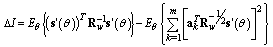 | (33) |
 . Therefore we have minimal value of
  if the subtrahend is maximal. Denote it
  . Inverting averaging with summation and taking into account the equality:
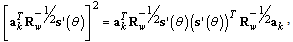 | (34) |
 | (35) |
 | (36) |
 takes place if
  are the orthonormal eigenvectors of the matrix
  , corresponding to
  largest eigenvalues
  and
and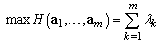 | (37) |
 implies trace of the matrix (36):
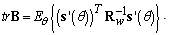 | (38) |
 . It implies:
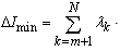 | (39) |
 is the m-dimensional subspace of the observation space with maximal Fisher information content about the parameter
  among any another m-dimensional subspaces.