1. Introduction

The computer time reduction for designing of large system is one of the sources of the total improvement of quality of designing. This problem has a great significance because it has a lot of applications, for example on VLSI electronic circuit design. Any traditional system design strategy includes two main parts: the mathematical model of the physical system that can be defined by the algebraic or integral equations and optimization procedure that achieves the optimum point of the objective function of design.

There are some powerful methods that reduce the necessary time for the circuit analysis. Because a matrix of the large-scale circuit is a very sparse, the special sparse matrix techniques are used successfully for this purpose[1]. Other approach for reducing the amount of computational required for both linear and nonlinear equations is based on the decomposition techniques. The partitioning of a circuit matrix into bordered-block diagonal form can be done by branches tearing as in[2], or by nodes tearing as in[3] and jointly with direct solution algorithms gives the solution of the problem. The extension of the direct solution methods can be obtained by hierarchical decomposition and macromodel representation [4]. Other approach for achieving decomposition at the nonlinear level consists on a special iteration techniques and has been realized in[5] for the iterated timing analysis and circuit simulation. Optimization technique that is used for the circuit optimization and designing gives a very strong influence on the total computer time too. The numerical methods are developed both for the unconstrained and for the constrained optimization[6] and will be improved later on. The practical aspects of these methods were developed for the electronic circuits designing with the different optimization criterions[7]. The fundamental problems of the development and adaptation of the automation designing systems were examined in some early papers[8,9].

The above described ideas of system designing can be named as the traditional approach or the traditional strategy because the method of analysis is based on the Kirchhoff laws.

The other formulation of the circuit optimization problem was developed on heuristic level some decades ago[10]. This idea was based on the Kirchhoff laws ignoring for all the circuit or for the part of the circuit. The special cost function is minimized instead of the circuit equation solving. This idea was developed in practical aspect for the microwave circuit optimization[11] and for the synthesis of high- performance analogue circuits[12] in extremely case, when the total system model was eliminated. The authors of the last papers affirm that the designing time was reduced significantly. This last idea can be named as the modified traditional design strategy.

Nevertheless all these ideas can be generalized to reduce the total computer time for the system designing. This generalization can be done on the basis of the control theory approach and includes the special control function to control the designing process. This approach consists of the reformulation of the total designing problem and generalization for obtaining a set of different designing strategies inside the same optimization procedure[13]. The number of the different designing strategies, which appear in the generalized theory, is equal to for the constant value of all the control functions, where M is the number of dependent parameters. These strategies serve as the structural basis for construction of different strategies with the variable control functions. However, the developed theory[13] is not the most general. In the limits of this approach only initially dependent system parameters can be transformed to the independent parameters but the inverse transformation is not supposed. The more general approach for the system designing supposes that initially independent and dependent parameters of system are completely equal in rights, i.e. any system parameter can be defined as independent or dependent one. In this case we have more vast set of the designing strategies that compose the structural basis.

2. Problem Formulation

In accordance with the new system designing methodology[13] the design process can be defined as the problem of the minimization of cost function for by the optimization procedure and by the analysis of the modified electronic system model. The optimization procedure can be determined in continuous form as:

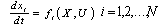(1)

The modified electronic system model can be expressed in the next form:

(2)

where N=K+M, K is the number of independent system parameters, M is the number of dependent system parameters, X is the vector of all variables ; U is the vector of control variables;;.

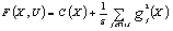
The functions of the right hand part of the system (1) depend on the concrete optimization algorithm and, for instance, for the gradient method are determined as:

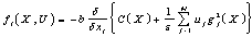(3)

where b is the iteration parameter; operator means ,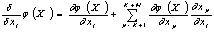

is equal to ; is the implicit function () that is determined by the system (2), C(X) is the cost function of the design process.

The problem of searching of the optimal algorithm of designing is determined now as the typical problem of the functional minimization of the control theory. The total computer designing time serves as the necessary functional in this case. The optimal or quasi-optimal problem solution can be obtained on the basis of analytical[14] or numerical[15-19] methods. By this formulation the initially dependent parameters for can be transformed to the independent ones when =1 and it is dependent when =0. On the other hand the initially independent parameters for , are independent ones always.

We developed in the present paper the new approach that permits to generalize more the above described designing methodology. We suppose now that all of the system parameters can be independent or dependent ones. In this case we need to change the equation (2) for the definition of system model and the equation (3) for the right parts.

The equation (2) defines the system model and is transformed now to the next one:

(4)

where J is the index set for all those functions for which u_i = 0, J = {j₁, j₂, . . .,j_z}, j_s with s = 1, 2, ..., Z, is the set of the indexes from 1 to M, = {1, 2,. .., M}, Z is the number of the equations that will be left in the system (4), Z ∈{0, 1. . ., M}. The traditional designing strategy (TDS) is defined by the control vector (11…100…0) with K units and M zeros, the modified traditional designing strategy (MTDS) is defined by the control vector (11…1) with N units. The right hand side of the system (1) is defined now as:

(5)

F(X,U) is the generalized cost function and is defined as:

(6)

This new approach for the process of designing was developed[20] in more generalized form than in[13]. It generalizes the methodology for the system designing and produces more representative structural basis of different strategies. The total number of different designing strategies, which compose the structural basis, is equal to . We expect the new possibilities to accelerate the designing process.

3. Numerical Results

New generalized methodology has been used for optimization of some non-linear electronic circuits. The numerical results correspond to the integration of the system (1) with variable step. The cost function C(X) has been defined as a sum of squares of differences between before defined and current value of some node voltages.

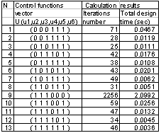
3.1. Example 1

In Figure 1 there is a three node nonlinear circuit.

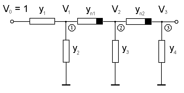Figure 1. Three-node circuit topology

This example includes seven parameters, i.e. four admittances and three nodal . The nonlinear elements were defined by the: , .

The vector X includes seven components: , , , , , , . The mathematical model of this circuit (4) includes three equations (M=3), and the functions are defined by the formulas:

(7)

The optimization procedure (1), (5) includes seven equations. The cost function C(X) is defined by the formula: .

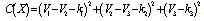
The total structural basis contains different strategies of designing. For instance, the structural basis of the previous developed methodology includes only different strategies. The designing results for all “old” strategies and for some of the new strategies are presented in Table 1.

Among the “old” strategies (14-21) there are three strategies (17, 18, and 21) that have the designing time lesser than the traditional strategy 14. However, the time gain is not very large. The best strategy 18 among all of the “old” strategies has the time gain 1.86 only. Nevertheless, among the new strategies we have some ones (2, 6, 10, 11, 12, 13) that have the design time significantly lesser than the TDS and they have the time gain more than 14. The optimal strategy among all of the presented strategies is the number 11. It has the computer time gain 23.1 times with respect to the traditional strategy of designing.

Table 1. Some Strategies of Structural Basis for Three-node Circuit

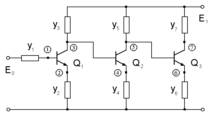
3.2. Example 2

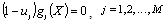
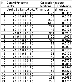
This example corresponds to the active network with transistor in Figure 2.

Figure 2. One-stage transistor amplifier

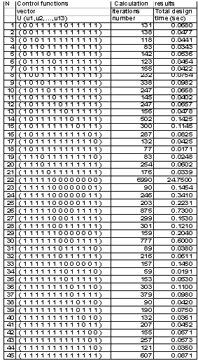
The Ebers-Moll static model of transistor has been used[21]. The vector X includes six components: , , , , , components: , , , , , . The model (4) of this network includes three equations (M=3), the optimization procedure (1) includes six equations (K+M=6).

The total “old” structural basis contains eight different strategies of designing. The total number of the different designing strategies that compose the new structural basis of the second level of generalized theory is equal to . The strategy that has the control vector (111000) is the TDS in terms of the first level of generalized methodology. In this case only three first equations of the system (1) are included in optimization procedure to minimize the generalized cost function F(X,U). The model of the circuit includes three equations too. The cost function C(X) was defined by 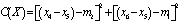, where are the before defined voltages on transistor junctions.

The strategy 16 that corresponds to the control vector (111111) is the MTDS. All six equations of system (1) are involved in the optimization procedure, but the model (2) has been vanished in this case. Other strategies can be divided in two parts. The strategies that have units for three first components of the control vector define the subset of “old” strategies. These are the strategies from 9 to 15 of Table 2.

Table 2. Some Strategies of Structural Basis for One-stage Amplifier

We can see that two strategies 12 and 14 have the total computer time lesser that others. Strategy 14 corresponds to the optimal one in this case and it has time gain 198 times with respect to the TDS. Strategies numbered from 1 to 8 are the “new” strategies of the second level of generalization. Strategy 2 has the minimal design time among all strategies and has more than twice time gain with respect to the best “old” strategy 14. The time gain achieves 404 times in this case. However, more impressive results were obtained analysing more complex networks.

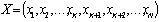
Figure 3. Three-node transistor amplifier

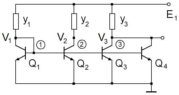
3.3. Example 3

In Figure 3 there is a transistor amplifier that has three independent variables as admittance (K=3) and three dependent variables as nodal voltages (M=3) at the nodes 1, 2, 3. The vector X includes six components, as for previous example. The control vector U includes six components .

The model of the circuit (4) includes three equations and the optimization procedure (1), (5) includes six equations. The cost function C(X) is defined by the formula: , where is a given collector current for the first transistor. The total structural basis contains different strategies. For instance, the structural basis of the previous developed methodology includes only different strategies. The results of the optimization process for some strategies for new structural basis and old structural basis are shown in Table 3.

Table 3. Some Strategies of Structural Basis for Example 3

Five last strategies are defined from the old structural basis and other strategies are from the new structural basis. As we can see the MTDS (number 13) is the best between both structural bases. The time gain of this strategy comparing with TDS is equal to 583. The new structural basis does not produce more fast strategies, but there many strategies that have time gain more than 100 times.

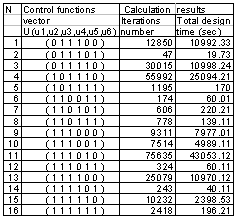
3.4. Example 4

The next example corresponds to the three-stage transistor amplifier in Figure 4.

Figure 4. Three-stage transistor amplifier

In this case the vector X includes 14 components. Seven components define the independent parameters , , , , , , and other seven components , , , , , , define the dependent parameters in accordance with the traditional approach. The cost function C(X) for the design problem was defined by the formula similar to the previous examples.

The structural basis consists of 128 different design strategies according to the first level of generalization. On the other hand the structural basis of the second level of generalization is equal to . Once again we have very broadened structural basis in the second case. The results of the analysis for some strategies of designing for this network are presented in Table 4. The designing strategies numbered from 12 to 25 belong to the subset that appears in limits of the first level of designing methodology.

Table 4. Some Strategies of Structural Basis for Three-stage Amplifier

The strategy 12 that corresponds to the control vector (11111110000000) is the TDS. The strategy 19 that corresponds to the control vector (11111111011111) has the minimum computer time among all the strategies of this subset. The time gain in this case is equal to 368 times. The strategies from 1 to 11 belong to the subset of new design strategies. Six strategies of this subset have the design time lesser than the best strategy of the “old” structural basis. The best strategy among new structural basis has the time gain 11715 times with respect to the TDS and has an additional time gain 31.8 times comparing to the better “old” strategy.

3.5. Example 5

The last example corresponds to the transistor amplifier in Figure 5.

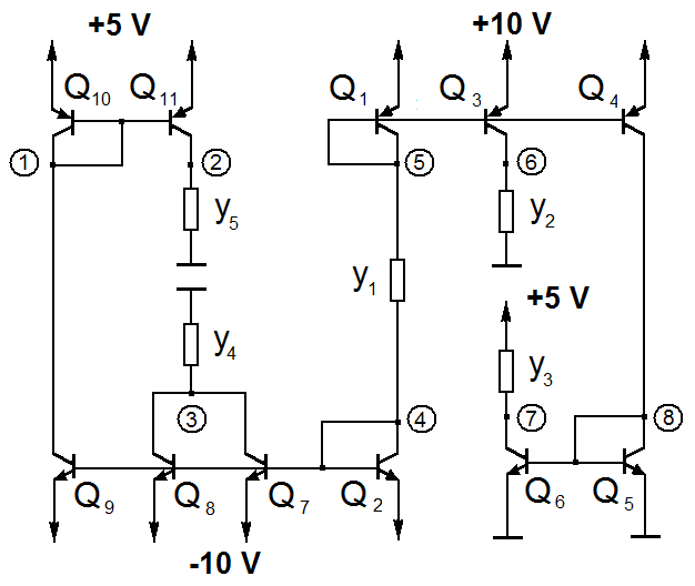Figure 5. Eight-node transistor amplifier

In this case the vector X includes 13 components. Five components define the independent parameters , , , , , and other eight components , , , , , , , define the dependent parameters in accordance with the traditional approach.

Table 5. Some Strategies of Structural Basis for Transistor Amplifier

The cost function C(X) for the designing problem was defined by the formula similar to the previous examples.

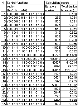
The structural basis consists of 256 different designing strategies according to the first level of generalization. On the other hand the structural basis of the second level of generalization is equal to . Once again we have very broadened structural basis in the second case. The results of the analysis of TDS and some strategies that have the designing time less than TDS are presented in Table 5.

The designing strategies numbered from 22 to 45 belong to the subset that appears on the basis of the first level of design methodology generalization. The strategy 22 that corresponds to the control vector (1111100000000) is the TDS. This strategy has a large number of iteration steps and a large computer time (24.75 sec). Other strategies that are presented in this table have considerably less iteration number and computer time. For instance the MTDS with control vector (1111111111111) has computer time 0.202 sec. The time gain in this case is equal to 123.7 times. The strategy 34 that corresponds to the control vector (1111111011110) has the minimum computer time among all the strategies of this subset. The time gain in this case is equal to 1295 times.

The strategies from 1 to 21 belong to the subset of new design strategies. Strategy 18 of this subset has the designing time lesser than the best strategy of the “old” structural basis. This strategy belong to the new structural basis and it has the time gain 1447 times with respect to the TDS and has an additional time gain 1.12 times with respect to the better strategy of the first level of the generalization.

Moreover among the “old” strategies there are 6 strategies that have the time gain more than 500 and 9 strategies that have the time gain more than 400. On the other hand among the “new” strategies there are 11 strategies that have the time gain more than 500 and 13 strategies that have the time gain more than 400.

So, taking into consideration the obtained results we can state that the second level of generalization of the designing methodology gives the possibility to improve all characteristics of the generalized design theory. Further analysis may be focused on the problem of searching of the optimal designing strategy by means of the control vector manipulation into the broadened structural basis. It is intuitively clear that we can obtain very great time gain by means of the new structural basis.

4. Conclusions

The traditional approach for the analogue circuit design is not time-optimal. The problem of the optimum algorithm construction can be solved more adequately on the basis of the optimal control theory application. The time-optimal designing algorithm is formulated as the problem of the functional minimization of the optimal control theory. The more complete approach for the electronic network designing methodology has been developed now. This approach generates the structural basis of the different strategies of designing that is more broadened than for the previous developed methodology. The potential gain of computer time that can be obtain on the basis of new approach is significantly more than for the previous developed methodology.

ACKNOWLEDGEMENTS

This work was supported by the Mexican Council of Sciences and Technology, under Grant CONACYT164624.