Musaab Hassan
Department of Mechanical Engineering, Faculty of Engineering, Sudan University of Science and Technology, Southern Campus, Khartoum, Sudan
Correspondence to: Musaab Hassan , Department of Mechanical Engineering, Faculty of Engineering, Sudan University of Science and Technology, Southern Campus, Khartoum, Sudan.
| Email: |  |
Copyright © 2012 Scientific & Academic Publishing. All Rights Reserved.
Abstract
Electromagnetic suspension system is commonly used in the field of high-speed vehicle, conveyor system, tool machines and frictionless bearing. Modelling a magnetic system requires modelling the magnetic force characteristics together with the current and the position. In this work; a 1D look-up table, of measured data, was used to represent the inductance as a function of the airgap. A 2D look-up table was generated to represent the electromagnetic force as a function of the current and the airgap. The proposed model account for both inductance variation and current variation as the airgap is changing.
Keywords:
Electromagnetic, Suspension, Inductance, Levitation Systems
1. Introduction
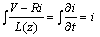
One of the main problems in modelling a magnetic suspension system is the nonlinearity inherent in the electromagnetic circuit. To model the magnetic levitation force, the force-position-current equation is often used[1,2,3, and 4]. Simulation data together with lookup tables was also implemented to model the system[5]. Experimental data which relate the force to the airgap is considered to be more realistic[6]. When applying a DC voltage into an electromagnet that is suspending an iron object (the object is freely suspended in the air), the voltage applied and the current induced in the circuit are related through the flux linkage as follows: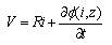 | (1) |
where;  is coil resistance,
  is the flux-linkage,
  is the current flowing in windings,
  is the time, and
  is the airgap.To model the full nonlinearity of the system, eqn.1 has to be used. There were various approaches to this problem discussed in[7] where different forms of equation.1 were applied. Methods carried out to handle the nonlinear data through mathematical approaches using curve fitting to represent the nonlinear data introduce some errors, and these errors will increase by the process of differentiation.
2. Modelling of a Magnetic Suspension System
The electromagnetic force is the rate of change of the co-energy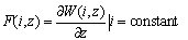 | (2) |
In the absence of leakage flux the same flux links the N-turn winding N times and also that the flux density is constant over the cross section, the magnetic co-energy can be written in the following form[8]; | (3) |
Assuming linear flux-current characteristics, the inductance can be written as[9], | (4) |
 is permeability of free space, N is the number of turns, and A is the cross sectional area .By substituting the inductance into energy equations, equation.2 can be written as follows;
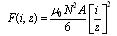 | (5) |
Nichols[10] used equation.5 to characterise an electromagnetic suspension system. In modelling electromagnetic system, equation.1 can be simplified as follow; | (6) |
 | (7) |
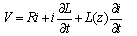 | (8) |
By ignoring the second term (assuming no variation in the inductance, so the first derivative is zero) and if the inductance variation according to the change in the airgap is taken into account, equation.8 can be written as follow: | (9) |
 | (10) |
Equation.10 will be used to model the system in MATLAB. Although the model doesn’t include the full nonlinearity of the system but it does allow for the inductance to be written as a function of the airgap, thus the equation deals with the nonlinearity partially.
3. Simulation Results and Discussion
A model using equation.10 was generated and implemented using MATLAB/SIMULINK software .The model is shown in Figure.1.A 1D look-up table was used to represent the inductance as a function of the airgap. A 2D look-up table was used to represent the electromagnetic force as a function of the current and the airgap. The values used in the 1D look-up table are measured data[10]. The output of the 2D look-up table is calculated using equation.5 while the two inputs (the current and the airgap) values within equation.5 are measured data[10]. The 1D look-up table reads out the inductance value corresponding to the given position input, while the 2D look-up table reads out the electromagnetic force corresponding to the given position and current inputs. The values used in the simulation model are given in Table.1[10], while Table.2 presents the measured data used in the 1D look-up table. The values used in the 2D look-up are plotted in Figure.2.| Table.1. values of variables used in the simulation[10] |
| | Quantity | Value | | Number of turns, N | 250 | | Measured system resistance, R | 10 Ω | | Pole face area, A | 0.003136 m2 | | Primary magnetic constant, μ o | 1.257*10-6 H/m | | Object mass, m | 0.2 Kg | | Gravity, g | 9.80665 m/s2 |
|
|
| Table.2. Measured airgaps values Vs. equivalent inductance[10] |
| | Z [m] | L (z) [H] | | 0.001 | 0.0821 | | 0.002 | 0.0411 | | 0.003 | 0.0274 | | 0.004 | 0.0205 | | 0.005 | 0.0164 | | 0.006 | 0.0137 | | 0.007 | 0.0117 | | 0.008 | 0.0103 | | 0.009 | 0.0091 | | 0.010 | 0.0082 |
|
|
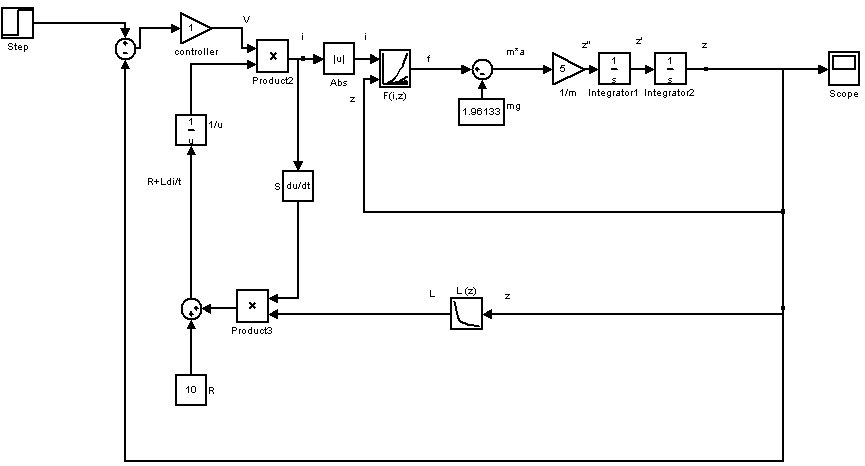 | Figure 1. Modelling system using equations. 5 & 10 |
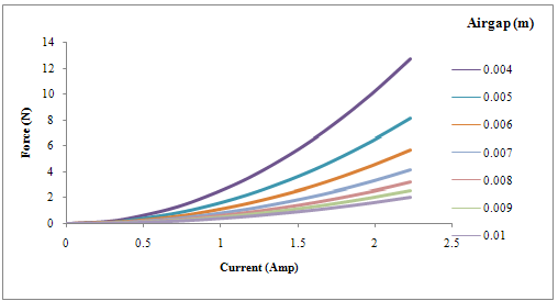 | Figure 2. the electromagnetic force at different airgaps and coil currents |
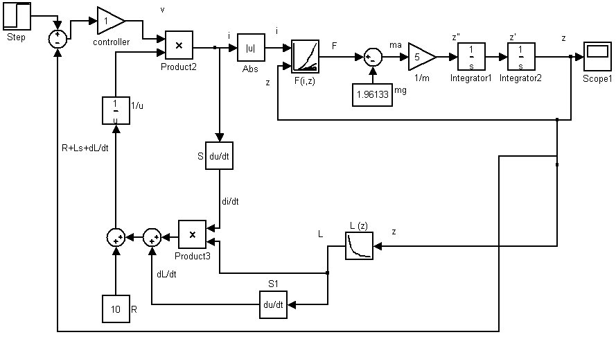 | Figure 3. Modelling electromagnetic suspension system using equation.8 |
The electromagnetic force will be used to suspend the iron object, thus: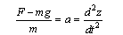 | (11) |
Where;  = acceleration. The acceleration was integrated twice to give the actual position.The magnetic suspension system is highly unstable. The position is fed back and compared with a reference position (nominal position) to form the error, and the error signal is used to derive the system. The model was run in MATLAB/SIMULINK and when applying a step response to the system, the airgap position is seen to fall down dramatically indicating instability.In the previous model, the derivative of the inductance was ignored which means that the term
  was set to zero. It is more realistic to represent the system using equation.8, which allows for the previous term to have values other than zero. Using equation.8, the model was improved as shown in simulation block diagram (Figure.3).The previous model was run in Simulink and the result showed instability of the system. This result is expected since the model contains no form of controller. The amounts of data used were quite enough (ten airgaps against eleven currents values which give a total of one hundred and ten values for the electromagnetic forces). The inductance table was generated at ten different airgaps. It is important to mention that the intermediate values which are not included in the tables are found by linear interpolation. Since a linear equation is used to generate the force and there were enough data used, the errors associated with interpolation are expected to be small. As time increases the airgap falls dramatically towards the negative values, which indicates that, the object will fall away from the electromagnet towards the earth gravity. This means that electromagnetic force applied is less than the gravity force and thus the object falls down.The differences between the two implemented models can be explained in terms of simplicity, amount of calculations, associated errors, and the degree of accuracy. The first model is simpler than the second model in term of the equation used to describe the system. Also, the second model is more descriptive in term of the nonlinearities, since the model allows for both current and inductance to vary according to the airgap. The amount of calculation performed, while simulating the system, in the second model is greater than that in the first model. That is due to the differentiation term added to the equation.
4. Conclusions
Two models were suggested and implemented to model the electromagnetic suspension system. A 1D look-up table was used to represent the inductance as a function of the airgap and a 2D look-up table was used to represent the electromagnetic force as a function of the current and the airgap. The second model is more accurate and representative but the amount of error is expected to be greater than that of the first model. This is due to the introduced differentiation process. At this stage, it is difficult to draw a conclusion regarding the exact behaviour of the system but the system is clearly unstable as the airgap is changing dramatically with time.
References
| [1] | ZG Sun, NC Cheung, JF Pan, SW Zhao, WC Gan, "Design and Simulation of a Magnetic Levitated Switched Reluctance Linear Actuator System for High Precision Applications" The IEEE International Symposium on Industrial Electronics (ISIE 2008) 30-June - 2 July, 2008, Cambridge, UK. |
| [2] | Barie, W. and Chiasson, J., ‘Linear and nonlinear state-space controllers for magnetic levitation’, International Journal of Systems Science 27(11), 1996, 1153–1163. |
| [3] | Khalid Ali, Mohammed Abdelati, Mohammed Hussein, “Modelling, Identification and Control of A Magnetic Levitation CE152”, Al-Aqsa University Journal (Natural Sciences Series), Vol.14, No.1, Pages 42-68, Jan.2010 |
| [4] | J. Van Goethem and G. Henneberger, "Design and implementation of a levitation-controller for a magnetic levitation conveyor vehicle", 8th International Symposium on Magnetic Bearing, Mito, Japan, August:26-28, 2002 |
| [5] | Y. S. Lee, J. H. Yang and S. Y. Shim, “A New Model of Magnetic Force in Magnetic Levitation Systems”, Journal of Electrical Engineering & Technology, Vol. 3, No. 4, pp. 584~592, 2008. |
| [6] | In-Gann Chen, Jen-Chou Hsul, Gwo Janm, Chin-Chen Kuo, Haw-Jer Liu, and M. K. Wu, “Magnetic Levitation Force of Single Grained YBCO Materials”, Chinese journal of physics vol. 36, no. 2, 1998 |
| [7] | J. M. Stephenson and J. Corda, “Computation of torque and current in doubly-salient reluctance motors from nonlinear magnetization data,” Proc. Inst. Elect. Eng., vol. 126, no. 5, pp. 393–396, 1979. |
| [8] | Jayawant, B.V., Electromagnetic Levitation and Suspension Techniques, Thomson Litho Ltd., 1981. |
| [9] | S. Colombi, A. Rufer, M. Zayadine, M. Girardin, Control Strategies for the Electromagnetic Levitated and Guided Vehicles of SwissMetro, MAGLEV 98: International Conference on Magnetically Levitated Systems and Linear Drives, Mt. Fuji, Japan.1998. |
| [10] | Nichol, Characterisation and control of electromagnetic suspension, Msc Thesis in Newcastle university, 1998. |
 Abstract
 Reference
 Full-Text PDF
 Full-Text HTML