Mohamed Bakry El_Mashade
Electrical Engineering Dept., Faculty of Engineering, Al Azhar University, Nasr City, Cairo, Egypt
Correspondence to: Mohamed Bakry El_Mashade , Electrical Engineering Dept., Faculty of Engineering, Al Azhar University, Nasr City, Cairo, Egypt.
| Email: |  |
Copyright © 2012 Scientific & Academic Publishing. All Rights Reserved.
Abstract
Optimum processor has received considerable attention in many areas of practical applications since it represents a reference tool against which the performance of any unknown processor is compared under any situation of operating conditions. As the performance of the processor under test closes to that of the optimum processor as it becomes more attractable. In the field of radar target detection, little attention has been paid to the performance evaluation of the optimum (fixed-threshold) detector. Therefore, it is of outstanding importance to analyze the performance of this detector in the more recent cases of environmental situations. Since the integration of M pulses represents one of the most important techniques that are used to improve the detection processing of a radar target, especially in nonideal environments, this manuscript is devoted to the performance evaluation of the fixed-threshold detection scheme when the radar receiver incorporates a video integrator amongst its basic elements to collect data from M-pulses in order to decide the presence or absence of the target under test which is assumed to be stationary or fluctuating. For fluctuating targets, the cases of noncoherent integration with fully-correlated, fully-decorrelated, and partially-correlated target returns are analyzed here. Additionally, incoherent integration of M-pulses, in which the consecutive sweeps themselves are correlated, is treated. In each case, closed form expression is derived for the detection performance of the detector under consideration given that its false alarm rate is held constant. The background noise and the successive pulses are assumed to be Gaussian stationary and fluctuating following χ2-distribution, respectively.
Keywords:
Optimum Detector, Noncoherent Integration, χ2-Distribution with K Degrees of Freedom, Partially- Correlated Targets, Nonfluctuating Targets
Cite this paper:
Mohamed Bakry El_Mashade , "Analytical Performance Evaluation of Optimum Detection of χ2 Fluctuating Targets with M-Integrated Pulses", Electrical and Electronic Engineering, Vol. 1 No. 2, 2011, pp. 93-111. doi: 10.5923/j.eee.20110102.15.
1. Introduction
The detection of signals in the presence of noise is one of the most basic and important problems encountered by communication systems designers. Although a great deal of work has been done in this area, most of this work has been based on the assumption that the signal and noise statistics are known. Although this is a reasonable assumption for many important problems, it is invalid for many others. Constant false alarm rate processors are useful for detecting radar targets in background for which all parameters in the statistical distribution are not known and may be nonstationary[1,14]. In most treatments of detection theory, emphasis is placed on the determination of optimal detectors requiring an essentially complete statistical description of the input signal and noise. There may be compelling reasons which lead toconsideration of other nonoptimal detectors. Amongst these reasons: a complete statistical description of the input may not be available, the statistics of the input data set may vary with time or may change from one application to another, and the optimal detector may be too complex to implement. Adaptive detectors have been developed to meet the first two conditions and can perform in a near optimal sense in an unknown or changing environment by proper adaptation of the detector structure[6,13].In most radar systems, there is relative motion between the radar and an observed target. Therefore, the cross section measured by the radar fluctuates over a period of time as a function of frequency and the target aspect angle. This observed radar cross section (RCS) is referred to as the radar dynamic cross section. This dynamic RCS may fluctuate in amplitude and/or phase. For most radar applications, phase fluctuations introduce linear error in the radar measurements, and thus they are not of a major concern. However, there are some cases, such as those require high precision and accuracy, where the phase fluctuation is detrimental. Amplitude fluctuations, on the other hand, can vary slowly or rapidly depending on the target size, shape, dynamics, and its relative motion with respect to the radar. Due to the wide variety of sources for these fluctuations, changes in RCS are modeled statistically as random processes[4].The fluctuation rate of a radar target may vary from essentially independent return amplitudes from pulse-to-pulse to significant variation only on a scan-to-scan basis. There are many distributions that can be used to characterize most target populations of interest. The Swerling models are a set of assumptions about the rate of target fluctuation relative to the pulse repetition frequency of a coherent radar system that employs noncoherent integration. Target amplitudes are Rayleigh distributed for SWI and SWII cases, while they have χ2-distributed for SWIII and SWIV models. From the correlation point of view, the correlation coefficient between the two consecutive echoes in the dwell-time is equal to unity for the SWI and SWIII cases while it equals zero for the SWII and SWIV models. In SWI and SWIII, the amplitude of the entire pulse train is assumed to fluctuate randomly from scan to scan; however, all pulses within a train have the same amplitude. The amplitude fluctuation is Rayleigh in the case of SWI model while it is of one dominant-plus-Rayleigh distribution in the SWIII fluctuation model. In SWII and SWIV, on the other hand, the amplitude of each pulse in the train is a statistically independent random variable with a Rayleigh or a one dominant-plus-Rayleigh probability density function, respectively[2,12].The χ2-distribution with 2κ degrees of freedom represents the sum of squares of "2κ" normally distributed random variables or the sum of the squared magnitudes of κ complex Gaussian random variables. It is more general than the Swerling models. In addition to Swerling and Marcum (nonfluctuating) models, the χ2-distribution includes the Weinstock model (κ<1), and the generalized model (κ a positive real number). On the other hand, the Rayleigh (SWI & SWII cases) model represents the χ2-distribution with two degrees of freedom (κ=1), while that with four degrees of freedom (κ=2) model contains (SWIII & SWIV cases). This family of models is used to represent complex targets such as aircraft and have the characteristic that the distribution is more concentrated about the mean as the value of the parameter κ is increased. It is often assumed that the Swerling cases bracket the behavior of fluctuating targets of practical interest. However, recent investigations of target cross section fluctuation statistics indicate that some targets may have probability of detection curves which lie considerably outside the range of cases which are satisfactorily bracketed by the Swerling cases. An important class of targets is represented by the so-called moderately fluctuating Rayleigh and χ2 targets, which when illuminated by a coherent pulse train, return a train of correlated pulses with a correlation coefficient in the range 0<ρ<1 (intermediate between SWII and SWI models in the case of Rayleigh targets) and (intermediate between SWIV and SWIII models in the case of χ2 targets)[7,10-11]. The use of moving target indicator (MTI) is useful in reducing the returns from stationary or slowly moving clutter However, its presence amongst the contents of the detection system complicates the analysis of that system since its output sequence is correlated even though its input sequence may be uncorrelated[3,5]. Therefore, it is of great importance to evaluate the performance of fixed-threshold detector in the case where the radar receiver employs MTI to detect moving targets.Our goal in this paper is to analyze the performance of the fixed-threshold algorithm for a target fluctuation model that obeys Swerling and Marcum models along with partially correlated χ2 targets with two and four degrees of freedom. Moreover, the performance of a radar signal processor that consists of a nonrecursive MTI followed by a square-law detector, a video integrator, and a fixed-threshold scheme is evaluated. In section II, the problem under investigation is formulated and the performance of the processor under consideration is evaluated for the standard Swerling models as well as the nonfluctuating model. The processor performance for moderately fluctuating χ2 targets with two and four degrees of freedom is analyzed, in section III. Section IV treats the problem of M-correlated sweeps and the performance evaluation of the fixed-threshold detector under such type of environmental conditions. In section V, we present a brief discussion along with our conclusions.
2. Statistical Background and Model Description
A radar echo is invariably immersed in additive noise and possibly in clutter return. Since noise and clutter are random phenomena, a decision concerning the presence or absence of a target is statistical in nature. In order to minimize the number of incorrect decisions, it seems reasonable to take advantage of a priori information concerning the echo signal structure and the statistical properties of the noise and clutter.The detection of a signal in noise can be formulated as a problem in hypothesis testing procedure in which the hypothesis that the received waveform doesn't contain a signal (H0) is to be tested against the hypothesis that the received waveform does contain a signal (H1). If the signal to be detected is deterministic that is its structure is completely known, then H1 is called a simple alternative. When the signal to be detected, on the other hand, is a member of finite or infinite set of signals, then H1 is called a composite hypothesis alternative.An essential feature of statistical decision detection theory is the decision rule used to arrive at a decision. The decision rule depends only on the observed waveform and not on signal. A decision rule that leads to decision d as a result of observation v is denoted by D(dv). The essence of the decision problem is to choose decision rules that accomplish the mapping of the points of the observation space into points in decision space with a pre-assigned probability in an optimum way with respect to a particular criterion of excellence[1].The Neyman-Pearson (NP) theory of hypothesis testing antedates the development of statistical decision theory. They define an optimum test as one that minimizes the probability of certain errors. In a test of hypothesis Hi, i=0 or 1, two types of errors can be made: H1 may be rejected when it is true, or it may be accepted when it is false. It seems reasonable that an optimum test should minimize the probability of committing both types of errors; that is the test should have a small probability of rejecting H1 when it is true and a large probability of rejecting H1 when it is false. The goal of the decision theory is to develop a criterion by which the most likely outcome could be selected. Since everything that is known about a random variable (RV) is contained in its probability density function (PDF), it is therefore of importance that the theory be formulated as a function of this PDF. Consider a sample point x in observation space defined by its PDF ƒ(x). The a priori density function for the null hypothesis is therefore written ƒ(xH0) and the simple alternative as ƒ(xH1). Now, if a single observation of x is made, which of the hypotheses can be assumed to be true? Defining the conditional probabilities P(H0x); which means H0 occurs given sample x, and P(H1x); which means H1 occurs given sample x. A decision rule can be formulated as follows: | (1) |
It should be noted that P(H0) and P(H1) are a priori probabilities, that are assigned as a result of prior knowledge. P(H0x) and P(H1x), on the other hand, are a posteriori probabilities, that are assigned after observations are made. Using the well-known relation that relates the joint probability density with the marginal and the conditional probability densities, Eq.(1) can be reformulated as: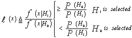 | (2) |
ℓ(x) is called the likelihood ratio. The above formula implies that there is a threshold value of x=T above which H1 is chosen and below which H0 is selected. This means simply that the decision criterion was to maximize the a posteriori probabilities given the a priori probabilities. However, additional information concerning the relative importance of the two hypotheses may have to be taken into account in forming the best decision strategy. The introduction of the cost or loss into the decision process allows us to carry out this task. If we associate a cost Cjk with each of the underlined joint probabilities, an average cost can be defined as: | (3) |
The problem is to minimize the average cost and obtain a likelihood ratio that includes cost. To obtain the desired ratio test, Eq.(3) needs to be written in terms of the PDF's ƒ(xH0) and ƒ(xH1). From the conservation of probability, we have 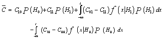 | (4) |
The likelihood ratio at x=t can be found by differentiating Eq.(4) with respect to t and setting the result to zero. This leads to | (5) |
According to Eq.(5), the decision rule can be formulated as | (6) |
In the case of a communication system, the a priori probabilities at the receiver are usually assumed to be equal. However, in the case of radar, the a priori knowledge of the signal statistics is generally unknown. Moreover, costs are generally difficult to assign in the radar problem. Therefore, it is required to determine the optimum threshold setting for a receiver if only the PDF's of the noise and signal-plus-noise are known. The NP solved this problem by maximizing the detection probability under the constraint of a prescribed false alarm probability. It is the decision process employed in most radar systems and is used as the baseline detection criterion in many applications. This rule doesn't require the a priori probabilities or cost functions.The decision rule to be developed minimizes the total type II error probability subject to the constraint of a fixed total type I error probability. Since the type II error probability is given by P(D0H1), the problem becomes one of maximizing the detection probability P(D1H1). The type I error, on the other hand, is the false alarm probability P(D1H0), which is chosen to be a constant determined by the noise statistics in the absence of the signal and the desired threshold setting. The average error probability to be minimized is then | (7) |
Here, the second term is a constant and doesn't affect the minimization process. However, the right side of Eq.(7) is equal to the average cost given by Eq.(3) under the substitutions C00=C11=0, C01P(H1)=1 and C10P(H0)=γ. Using the solution given by Eq.(5) with the values of Cjk above leads to evaluating the unknown Lagrange multiplier γ which becomes equal to the likelihood ratio at x=t. The threshold setting T follows simply from the false alarm probability Pfa= P(D1H0) after replacing t by T. Thus, | (8) |
The corresponding detection probability Pd = P(D1H1) is given by | (9) |
Fig.(1) shows the block diagram of the resulting detection scheme. Here, we consider a radar system in which time diversity transmission is employed and assume that M pulses hit the target. The receiver model has a white Gaussian noise, which is independent from pulse to pulse. The received IF signal is applied to a matched filter, which is specifically designed to maximize the output signal-to-noise ratio.The output of this filter is then passed through a square- law device to extract the baseband signal. This signal is then sampled and the sampling rate is assumed to be such that the samples are statistically independent. The square-law detected video range samples are then compared to the pre- assigned detection threshold to decide whether the target is present or absent.
3. Multipulse Analysis of Optimum Detector
3.1. Swerling Models
Time diversity transmission is often used to circumvent the high probability of a deep fade on a single transmission which may result in loss of the signal. One way to combat deep fades is to postdetection integrate the received observations from each range resolution sample. The final decision, about the presence or the absence of a target, is made by comparing the integrated signal to a threshold. In this case, the signal and noise are represented by vectors; each one of them has M components. The components of each vector are uncorrelated as well as the components of the noise vector are uncorrelated with those of the signal vector.When the input time sequence to the square-law detector is normally distributed, its output obeys the exponential PDF with parameter μ[6]. Thus, | (10) |
U(x) denotes the unit step function. Under the null hypothesis of no target in a range cell and homogeneous background, μ represents the total clutter-plus-thermal noise power, which is denoted by "ψ". Under the alternative hypothesis of the presence of a target, on the other hand, μ is replaced by ψ(1+α) ; with "α" being the average SNR of the target. The replacement of the PDF in the definitions of false alarm and detection probabilities, Eqs.(8,9) with that given in Eq.(10) yields  | (11) |
Fq(.) represents the cumulative distribution function (CDF) associated with the random variable q, which represents the cell under test (CUT). From the above expression, it is obvious that the CDF of the CUT is the backbone of the analysis of the fixed-threshold detector. In the case of noncoherent integration of M pulses, the CUT is composed of M samples; each one of them belongs to one pulse of the successive train of pulses. Thus, the CUT is represented by a RV "Q" created by the summation of M random variables qi's as: | (12) |
Since each of the random variables qi’s has an exponential distribution, Eq.(10), Q has a gamma distribution for its PDF[13]. Thus, | (13) |
 | Figure 1. Architecture of fixed threshold detector with postdetection integration |
In the above expression, Γ(M) denotes the gamma function. The CDF associated with the above PDF is[14] | (14) |
For our analysis to be generalized, the χ2-distribution must be considered. If  denotes the average M-pulse SNR, the PDF of the target return when it is fluctuating obeying χ2-distribution is[4]:
 | (15) |
Where 1F1(.) represents the confluent hypergeometric function. The above expression represents the PDF of the sum of the squares of 2κ = K Gaussian random variables where κ denotes the degrees of freedom of this distribution. The CDF associated with this PDF becomes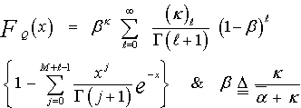 | (16) |
In the above expression, (κ)j denotes the Pochhammer symbol which is defined as: | (17) |
The four well-known cases of Swerling model can be deduced from this relation by choosing the degrees of freedom κ as; | (18) |
Once the CDF of the tested cell is calculated, the processor detection performance becomes completely determined, as Eq.(11) states. It is of importance to note that the selection between the probability of false alarm and that of detection is based on the SNR parameter ( ) which in this case represents the absence (
 =0) or the presence (
 ≠0) of the radar target.
3.2. Partially-Correlated χ2 Targets
The classical models of Swerling for target echo fluctuation are not practically sufficient to represent most of the radar target fluctuation. There is an important class of these fluctuation models which is known as moderately fluctuating targets. The illumination of this class of radar targets by a coherent pulse train, return a train of correlated pulses with a correlation coefficient in the range 0<ρ<1 (intermediate between SWII and SWI models in the case of Rayleigh targets) and (intermediate between SWIV and SWIII models in the case of χ2 targets). In this case, it is important to note that the components of the noise vector remain the same as in the previous case, while the components of the signal vector are correlated with each other with a correlation coefficient ρ and the signal's vector components still uncorrelated with those of the noise vector, as in the case of Swerling fluctuation models. The detection of partially correlated χ2 targets with two (κ=1) and four (κ=2) degrees of freedom is therefore of great importance As shown in[11], the MGF of the radar target that is fluctuating following χ2 with two (K=2) degrees of freedom is given by | (19) |
On the other hand, for χ2- fluctuation model with four (K=4) degrees of freedom is[12] | (20) |
In the above formulas, λi’s are the nonnegative eigenvalues associated with the correlation matrix Λ. In view of Eqs.(19 & 20), the solution for partially correlated case requires the computation of the eigenvalues of the correlation matrix Λ. To calculate these eigenvalues, it is assumed that: i- the statistics of the signal are stationaryii- the signal can be represented by a first order Markov process. Under these assumptions, Λ is a Toeplitz nonnegative definite matrix, the general form of which can be written as:  | (21) |
Since the calculation of the CDF of the target return is the backbone of the processor performance determination, let us go to evaluate it for the MGF's given in Eqs.(19, 20). To carry out this task, it is well-known that there is a direct relation between the transformation of the CDF and the MGF, to which it is associated, according to | (22) |
Where | (23) |
The Laplace inverse of the above formula results in the required CDF. Thus, | (24) |
with | (25) |
and | (26) |
with  | (27) |
and | (28) |
Once the CDF of the CUT is computed, the fixed- threshold detector becomes completely evaluated as Eq.(11) demonstrates.
3.3. Numerical Results
Let us now go to carry out the numerical evaluation of the previous derived formulas on a PC to show the reliability of the mathematical formulation of the optimum detector performance and to see to what extent they are valid. Since the detection threshold represents the backbone of this performance and its selection is more sensitive to the required rate of false alarm, we start our calculations with this important parameter. Fig.(2) displays the detection threshold "T" in dB as a function of false alarm probability for different numbers of noncoherently integrated pulses. Since the optimum processor is of fixed-threshold type of detection techniques, once its threshold is setting, it is held unchanged either the environmental circumstances remain stationary or fluctuate with time. In other words, the optimum processor assumes always that the operating environment is ideal without any nonhomogeneities. The results of this figure illustrate that as M increases, the detection threshold increases.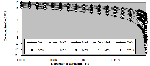 | Figure 2. M-sweeps detection threshold as a function of false alarm probability of fixed threshold detector for 2 fluctuating targets |
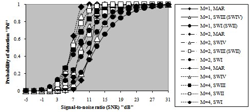 | Figure 3. M-sweeps detection probability, as a function of the target signal-to-noise ratio of the fixed threshold detector for2 target fluctuation model |
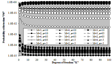 | Figure 4. M-sweeps detection performance of fixed threshold processor for2 fluctuating targets with K degrees of freedom |
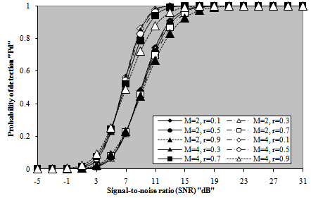
The correspondence between M and T can be explained as follows: as M increases, the effective value of the cell under test (CUT) increases and since the false alarm rate is kept constant, the detection threshold must be raised for the false alarm rate to be kept at its designed value without any changes. On the other hand, T decreases as the false alarm rate increases. This is because there is a strong correspondence between the false alarm probability and the integration interval. As the rate of false alarm increases, the integration interval increases and consequently the detection threshold decreases, given that the number of integrated pulses (M) is held constant. In the limit, the detection threshold tends to zero as the false alarm rate tends to one. In this situation of operating conditions, all the detection decisions of the processing scheme are false. This behavior is common either the processor makes its detection decision based on single-sweep data or collects data from M-sweeps. Once the detection threshold is setting, it is of importance to show the effect of the strength of the target return on the detection performance of the processor under consideration. Since this threshold is a function of false alarm rate, we perform our numerical results for a false alarm probability of 10-6 which is held constant throughout this research. Fig.(3) depicts the detection performance of the optimum scheme as a function of the strength of the signal returned from the target to be detected for several values of noncoherently integrated pulses when the target under test is either stationary or fluctuating in accordance with SWI, SWII, SWIII, and SWIV. The candidates of this figure are parametric in M as well as the fluctuation model of the target to be detected. It is of importance to note that the label MAR on a specified curve indicates that it is drawn for a stationary or Marcum model for the tested target. For weak SNR, the SWI fluctuation model gives the highest detection probability, the SWIII comes next, after that the SWII model reserves its tour, and the SWIV fluctuation case has the lowest value of detection probability. This classification is according to the Swerling fluctuation models. However, the nonfluctuating (stationary) model gives generally the worst detection performance in this region of operating SNR. On the other hand, as the returned signal from the radar target becomes strong, the reverse of the above classification takes place. This means that the stationary model has the highest detection performance and the SWI fluctuation model presents the worst value of detection probability. For M=2, the SWII and SWIII fluctuation models give identical performances, as the theoretical analysis demonstrates. Additionally, the target fluctuation models SWI and SWII have the same detection behavior in the absence of noncoherent integration (M=1). Moreover, the χ2-fluctuation models with four degrees of freedom (SWIII & SWIV) present identical detection performances in the case of single sweep source of data. The curves of monopulse case are included amongst the candidates of this figure as references against which the M-sweeps numerical results are compared to show to what extent the detector performance can improve with noncoherent integration of M pulses. It is shown that as M increases, better detection performances are obtained and lower SNR values are required to attain a pre-assigned level of detection. Due to the important role that the degrees of freedom of χ2-fluctuation model can play in determining the processor detection performance, Fig.(4) is devoted to present the variations of detection probability with this important parameter for constant levels of signal strength in the absence as well as in the presence of noncoherent integration. For each number of integrated pulses, three values of SNR (α=-5, 5, and 10dB) are chosen to demonstrate the previous concluded remarks from the presentation of Fig.(3). For weak level of signal strength (α=-5dB), the probability of detection attains its maximum value for lower values of degree of freedom (Κ=1) and it decreases monotonically till Κ=10 after which it remains constant without any changes. For moderate level of signal strength (α=5dB), on the other hand, the same behavior is anticipated with the exception that the processor gives higher level of detection relative to the case where the target return is weak. As the strength of the returned signal increases (α=10dB), the processor performance improves and the detection probability reaches a value which is higher than that attained for α=5dB and rests unchanged whatever the degree of freedom is. When the target signal becomes strongest, the reverse of the processor reaction against weak level of signal strength is demonstrated. This means that the detection performance reaches its lowest value at Κ=1 after which it increases monotonically till it attains its maximum value after which it rests constant regardless of the degree of freedom. After this brief discussion about the results of monopulse case, let us consider the multipulse case. As M augments, the single-sweep behavior is observed with some improvements in the detection performance for each case of the three selected levels of signal strength. As we have previously stated, lower levels of SNR are required to achieve a predetermined level of detection as the number of noncoherently integrated pulses increases. The behavior of curves of Figs.(3-4) confirms this predictable remark. Now, we will go to calculate another important characteristic of the fixed-threshold detection scheme. This interesting parameter is known as receiver operating characteristic (ROC) in radar terminology. This parameter describes the variation of the detection probability with the rate of false alarm for a given level of signal strength when the radar receiver noncoherently integrates M pulses to establish its detection threshold in order to decide the presence or absence of stationary or fluctuating radar target. The obtained numerical results of this parameter are displayed in Fig.(5) for a signal level of 5dB. This value of α is chosen low in order to prove the validity of the concluded remarks which are extracted from the results of the previous figures. For low rate of false alarm, the SWI fluctuation model has the highest detection performance and as the false alarm rate increases, its superior behavior is quickly reversed to be the worst one for higher rates of false alarm. The SWIII model comes in the next class in both regions of operating false alarm rate. Then the SWII fluctuation model reserves its third place, the SWIV model follows it and finally the nonfluctuating model which gives the worst detection performance in the region of lower rates of false alarm and the highest detection probability for higher values of false alarm rate. When the probability of false alarm is low, the detection threshold is high and for the detection scheme to be sensitive to the target signal, the successive returns must be highly correlated. Therefore, the SWI and SWIII fluctuation models have the best detection performance. Since the strength of correlation increases as the degree of freedom decreases, the SWI model has a detection behavior which exceeds that of the SWIII model given that the false alarm rate is held low. As the rate of false alarm increases, the detection threshold decreases correspondingly and the reverse manner of the previous sequence is observed. In other words, when the detection threshold decreases, the area, to be integrated, under the distribution of the received signal increases and consequently the processor detection performance will be improved. In this case, the effective value of the signal, to be compared with the detection threshold, increases as the correlation between the successive returns decreases and attains its maximum value in the case where these returns become uncorrelated. Hence, SWII model gives higher performance than SWI, and the detection performance of SWIV model exceeds that of SWIII model. In addition, as the degree of freedom increases, the signal's effective value increases and consequently the processor performance improves, given that the signal's strength is of considerable level. Therefore, the SWIII fluctuation model given higher performance than that of SWI model although the successive returns are fully correlated in both cases and the superiority of the SWIV model exceeds that of the SWII although the successive returns are uncorrelated. Since the target cross-sectional area is fixed in the successive returns in the case of stationary target, this model has the highest detection performance in the region of large values of false alarm rate and it has the worst detection behavior in the region where the false alarm is held at low rate owing to the resulting threshold in each case. In all cases, there is an improvement, relative to the single-sweep case, in processor performance when the radar receiver incorporates a video integrator amongst its basic elements and this improvement increases as the number of noncoherently integrated pulses increases.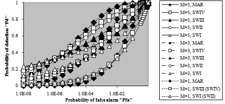 | Figure 5. M-sweeps receiver operating characteristics (ROC's) of fixed-threshold scheme for 2 target fluctuation model when the strength of the target signal (SNR) is 5dB |
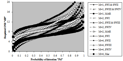 | Figure 6. M-sweeps required signal-to-noise ratio (SNR), in dB, to achieve an operating point (1.0E-6, Pd) of fixed-threshold detector for 2 target fluctuation model |
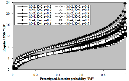
Let us turn our attention to another category of numerical results that measure the goodness of the processor performance. This category is concerned with searching of the required SNR to achieve a pre-assigned level of detection given that the false alarm rate is taken constant. Fig.(6) depicts the variation of the necessary SNR, to attain the required probability of detection, as a function of the demand level of detection for a constant false alarm probability of 10-6 when the target under consideration is either stationary or fluctuating following Swerling models in the absence (M=1) as well as in the presence of noncoherent integration (M>1). For low values of detection level, the required SNR increases linearly with a noticeable rate of increasing till the pre-assigned probability of detection reaches 10% after which the rate of increasing becomes relatively low and continues in this manner till the required level of detection attains 90% beyond which the required SNR augments rapidly with the demand probability of detection. The inclusion of the monopulse results amongst the candidates of the current figure is for the purposes of comparison. An accurate vision on the behavior of the curves of this figure indicates that the stationary model has the lowest rate of increasing in all the three distinct regions of the required level of detection, while the SWI fluctuation model gives the highest rate of increasing in each one of these regions. In other words, the behaviors of the nonfluctuating and the SWI models embrace those of other models considered in this manuscript. This means that the Marcum model requires the highest SNR to achieve a pre-assigned level of detection given that this level is weak (Pd<30%), and the SWI model requires the lowest value of SNR under the same conditions of operation. On the other hand, as the demand level of detection becomes stronger, the reverse behavior is exactly observed. In each one of these situations, the SWII, SWIII, and SWIV fluctuation models necessitate intermediate values of SNR that lie between these two extremes. Additionally, as M increases, lower SNR values are required to respond the necessary level of detection whether the target under test fluctuating or nonfluctuating. It is of interesting to note that the SWI and SWII models have identical behavior in the absence of noncoherent integration (M=1). Also, the behaviors of SWIII and SWIV fluctuation models are the same under single-sweep case. Moreover, the behavior of SWIII model, under noncoherent integration of two pulses (M=2), is a copy of that corresponding to SWII fluctuation model.The computation of the required SNR to respond the demand level of detection is very interesting, especially, if the problem under consideration is associated with the radar target detection. After the calculation of the SNR necessary to achieve any level of detection, let us now go to fix the level of detection at acceptable value (Pd=90%) and research for the SNR value that is capable to carry out this task when the degrees of freedom (Κ) of the χ2- fluctuation model vary from one to infinity, given that the radar receiver contains a postdetection integrator amongst its basic contents and the false alarm rate is held constant at 10-6. The obtained results are illustrated in Fig.(7) which plots the required SNR against Κ for a number of integrated pulses of 2, 3, 5, 7, and 9 along with the single-sweep curve as a reference against which the M-sweeps curves are compared. This presentation demonstrates the role that the parameter Κ can play on the behavior of the radar system of detection. It is obvious that the required SNR decreases rapidly with the degrees of freedom till Κ=4 after which it is slowly decreasing until Κ=20 beyond which it rests approximately unchanged. This behavior is common for any number of integrated pulses with the exception that as M increases, lower values of SNR are required to reach the required level of detection. The last presentation concerning the evaluation of the SNR is associated with the variation of this important parameter as a function of the number of integrated pulses M taking into account that the demand level of detection is held fixed at the previous chosen value of 90%. Fig.(8) displays this evaluation for two constant rates of false alarm (10-8&10-6). The independent parameter of this plotting represents the number of noncoherently integrated pulses which varies from 2 to 15 in addition to the fundamental monopulse (M=1) situation. The behavior of the curves of this figure sustains our extracted notes about the processor performance which is simultaneously examined against postdetection integration and the situation of the radar target from the stationarity point of view. The new contribution of the present figure is to show to what extent the required SNR raised as the demand rate of false alarm is lowered to reach 10-8 which is practically attractable given that the detection level is kept constant. For M=1, the optimum processor requires a SNR of 22.4dB to achieve an operating point of Pfa=10-8 and Pd=90%, while it demands a SNR of 21.1dB to achieve the same level of detection except that the rate of false alarm augments to 10-6, given that the radar target fluctuates in accordance with χ2-model with two degrees of freedom. If the radar receiver integrates 15 successive pulses, the corresponding values to the above stated rates of false alarm are 13.3dB and 12.3dB, respectively, when the target fluctuates following SWI model, while they are 5.6dB and 4.75dB, respectively, when the fluctuation model of the target under test follows SWII model. This example demonstrates the utility of pulse integration in improving the performance of the radar system of detection. However, as M increases, the complexity of the constructed system increases in addition to increase the processing time taken by the system in formulating the decision of detection. Practically, a compromise factors are taken into account in choosing the number of integrated pulses and the complexity of the detection system in such a way that the implemented system becomes as simple as possible in addition to formulate its decision as fast as possible and in a very accurate manner. 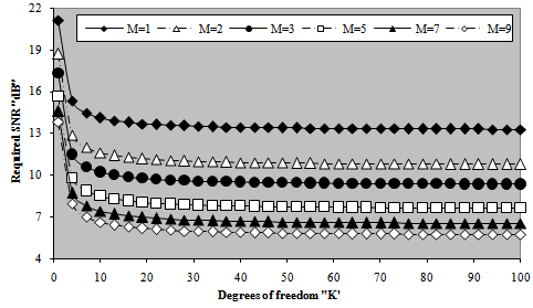 | Figure 7. M-sweeps required signal-to-noise ratio (SNR), to achieve an operating point of (1.0E-6, 0.9), against degrees of freedom K of fixed- threshold detector for 2 fluctuating targets |
 | Figure 8. M-sweeps required SNR to achieve an operating point (Pfa, Pd), against number of integrated pulses of fixed-threshold detector for 2 fluctuating targets |
 | Figure 9. M-sweeps detection performance of fixed threshold processor for partially-correlated 2 target fluctuation model with 2-degrees of freedom |
 | Figure 10. M-sweeps detection performance of fixed threshold processor for partially- correlated 2 target fluctuation model with 4-degrees of freedom |
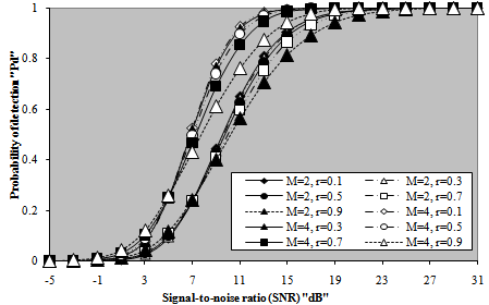
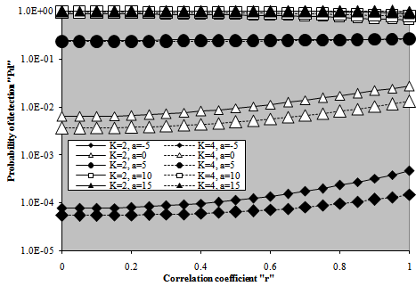
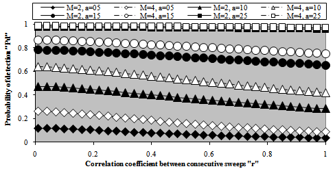
Till now, we are concerned with target returns which are fully correlated (SWI & SWIII cases) or fully decorrelated (SWII & SWIV cases), from the fluctuation point of view. The next category of presentation is associated with the evaluation of the performance of fixed-threshold detector for partially correlated χ2 fluctuating targets. This category comprises Figs.(9-10). In these figures, the detection probability is plotted as a function of the radar target signal strength and parametric in the correlation coefficient between the target returns when this target fluctuates following χ2-model with two and four degrees of freedom, respectively, and for a number of integrated pulses of 2 and 4. The curves of these figures are labeled in the number of postdetection integrated pulses, M, and the correlation coefficient between the target returns (ρ). From the results of these figures, it is observed that as the correlation between successive returns increases, the processor performance becomes more degraded. In addition, for low SNR, the processor performance improves as the correlation coefficient between consecutive sweeps increases and this behavior is rapidly inverted as the strength of the target signal becomes stronger. Moreover, as the number of noncoherently integrated pulses increases, the processor performance improves and less SNR value is needed to attain the same level of detection. Additionally, the processor performance for χ2-fluctuation model with four degrees of freedom (K=4) exceeds that for χ2-model with two-degrees of freedom (K=2) under the same conditions of operation. In both cases, the degradation in detection performance is negligible when the successive returns are weakly correlated, while it is significantly clear for highly correlated returns. The results of these figures demonstrate that the processor performance improves as the number of degrees of freedom ‘Κ’ increases, given that the correlation coefficient ‘ρ’ is held constant. To illustrate the influence of the signal correlation on the processor detection performance, the detection probability is plotted against ρ for different levels of signal strength when the fluctuation of the radar target follows χ2-model with 2- and 4-degrees of freedom. This plotting is shown in Fig.(11) for the case where the radar receiver integrates two pulses (M=2) before formulating its detection decision. The family of curves of this figure is labeled in the degrees of freedom (Κ) of the target fluctuation model in addition to the signal strength (α).For weak signal strength (α=-5dB), the processor performance improves as the target returns become strongly correlated, as we have previously shown. This behavior is valid till the target return becomes stronger en face of noise (α=10dB) after which the normal behavior takes its place. The normal behavior in this text means that the processor performance degrades as the correlation coefficient between consecutive returns increases. From this presentation, we conclude that the processor performance increases with ρ when the strength of the target return is weak, while this performance becomes worsen, as ρ increases, for stronger target signal. On the other hand, Fig.(12) shows the same characteristics for a number of integrated pulses of 4. Examining the candidates of this plot demonstrates that they have the same characteristics as those of Fig.(11) except that the level of the signal strength at which the processor alters its behavior is lowered.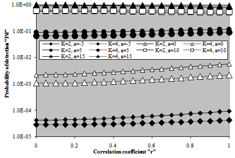 | Figure 11. M-sweeps detection probability versus correlation coefficient between consecutive sweeps of fixed threshold detector for partially-correlated 2 targets when M=2 |
 | Figure 12. M-sweeps detection probability versus correlation coefficient between consecutive sweeps of fixed threshold detector for partially- correlated2 targets when M=4 |
 | Figure 13. M-sweep required SNR, to achieve an operating point of (1.0E-6, 9.0E-1), as a function of consecutive sweeps correlation coefficient of fixed-threshold detector for 2 fluctuating targets |
 | Figure 14. M-sweeps required SNR, to achieve an operating point of (1.0E-6, Pd), of fixed-threshold detector for partially-correlated 2 targets |
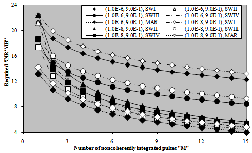
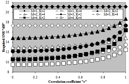
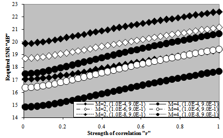
The last category of curves associated with the partially- correlated χ2-fluctuating targets is concerned with the calculation of the required SNR to attain a specified level of detection, either this level is fixed throughout the entire candidates of the figure as in the case of Fig.(13), or vary as in the case of Fig.(14), given that the false alarm rate is kept constant at 10-6. The examination of the curves of Fig.(13) illustrates that they are classified into two separate families. The first family depicts the variation of the calculated SNR with the correlation coefficient between the consecutive target returns when this target fluctuates following χ2-model with two-degrees of freedom, while the second family represents the same thing in the case where the radar target fluctuation obeys χ2-model with four-degrees of freedom. As predicted, the χ2-fluctuation model with 4-degrees of freedom requires less level values, in comparison with that of 2-degrees of freedom, for signal strength (SNR) to achieve the needed level of detection given that the operating circumstances are kept the same in the two cases. The monopulse results, which are independent of the correlation coefficient, are included in this figure as a reference to see to what extent the necessary SNR, to verify an operating point of (Pfa=1.0E-6, Pd=9.0E-1), decreases with integration of M-pulses. It is obvious that as ρ increases, there is a small increasing in the required SNR till ρ reaches 80% beyond which the rate of increasing becomes significantly noticeable. Additionally, the χ2-model with higher degrees of freedom needs lower values of SNR than that with lower degrees of freedom on the condition that the operating environment is the same in the two cases. Moreover, the rate of increasing of the χ2-model with higher degrees of freedom is lower, even in the region where the correlation between the consecutive returns becomes stronger (ρ≥80%), than that in the case of χ2-model with lower degrees of freedom. It is of outstanding importance to note that the required signal strength for the detection processor to achieve a specified level of detection decreases by increasing either the degree of freedom of the χ2-model or the number of noncoherently integrated pulses, or increasing both of them. The results of Fig.(14), which is an alternative version of Fig.(13), ), support these concluded remarks. In this situation, the necessary SNR to attain a specified value of detection probability is drawn against the needed level of detection on the condition that the false alarm probability is fixed at 10-6. The candidates of this figure are parametric in M, Κ, and ρ. The insight vision on the behavior of the curves of the figure demonstrates that there are two groups of these curves: one of them represents the results for two integrated pulses, while the other denotes those when the radar receiver noncoherently integrates four pulses. Each one of these groups has a common point at which the calculated SNR is approximately constant regardless of the level of correlation or the degree of freedom. This point corresponds to 27% and 31% levels of detection for M=2 and 4, respectively. For probability of detection values less than the critical value, the required SNR decreases as either ρ increases or Κ decreases. As the detection level exceeds the critical level, the behavior of the curves is reversed, i.e. the necessary signal strength to attain a given level of detection decrease as either the strength of correlation between consecutive returns decreases or the degree of freedom of the χ2-fluctuation model increases. Either the operating region is, the rate of change of the computed SNR increases as the distance from the critical point increases. Additionally, as M increases, the critical point shifts towards higher level of detection and the detection scheme demands lower signal levels in order to perform a pre-assigned level of detection.
4. Performance of Optimum Detector Processing M-Correlated Sweeps
4.1. Detector's Structure
Clutter is a term used to describe any object that may generate unwanted radar returns that may interfere with normal radar operations. It can be classified in two categories: surface clutter and volume clutter. Surface clutter includes trees, vegetation, ground terrain, man-made structures, and sea surface. It manifests in airborne radars in the look-down mode. It is also a major concern for ground-based radars when searching for targets at low grazing angles. Volume clutter, on the other hand, has large extent and includes chaff, rain, birds, and insects. It consists of a large number of small dipole reflectors that have large radar cross section values. It is released by hostile aircraft or missiles in an attempt to confuse the defense. Surface clutter changes from one area to another, while volume clutter may be more predictable[4].The power spectrum of stationary clutter is concentrated around DC (f=0) region. However, clutter is not always stationary; it actually exhibits some Doppler frequency spread because of wind speed and motion of the radar scanning antenna. Therefore, the clutter power spectrum can be represented as the sum of fixed (stationary) and random components. Nevertheless most of the clutter power is lumped around zero Doppler with some spreading, it is modeled by Gaussian-shaped power spectrum with its mean at zero in addition to integer multiples of the pulse repetition frequency.Since clutter represents an unwanted signal, it is customary needed to avoid or reduce it to a large extent as possible. In continuous wave radars, clutter is avoided or suppressed by ignoring the receiver output around DC, since most of the clutter power is found in that region. Pulsed radar systems may utilize special filters that can distinguish between slowly moving or stationary targets and fast moving ones. This class of filters is known as moving target indicator (MTI). In other words, the MTI filter is introduced to suppress target-like returns produced by clutter and allow returns from moving targets to pass through with little or no degradation. However, the presence of MTI complicates the analysis of the detection system performance since its output sequence is correlated even though its input sequence may be uncorrelated. In the reminder of this section, our scope is to evaluate the performance of the fixed-threshold detector when it is incorporated in a radar receiver with MTI filter. The block diagram of the system to be analyzed is shown in Fig.(15). For M consecutive sweeps with sweep-to-sweep correlation coefficient ρℓk, the correlation matrix of the integrator output takes the form[5]: | (29) |
The previous matrix can be diagonalized by means of an orthogonal transformation which is determined by the solution of its associated eigenvalue problem. The resulting eigenvalues (λi's) and eigenvectors ( 's) determine the interferences and the signal gains, respectively. In terms of these important parameters, the MGF of the integrator output for the target cell Q has a form given by[3]
 | (30) |
Where | (31) |
In the above formulas, gj denotes the jth signal gain corresponding to the jth eigenvector. ψ represents the total clutter-plus-thermal noise power, α indicates signal-to-noise ratio (SNR) of the target under test. This means that the returns from the primary target fluctuate in accordance with Swerling I model[5].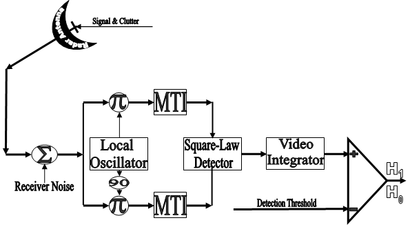 | Figure 15. block diagram of fixed-threshold detector with incoherent integration |
In order to analyze the performance of the processor under consideration, it is required to obtain the t-domain representation of Eq.(28), i.e., the PDF of the content of the cell under test Q. To carry out this inverse, Eq.(28) can be formulated in another simpler form as: | (32) |
The coefficients ci's are functions of λi,  , gj, and α. If the roots of this Mth order polynomial are determined, either analytically or numerically, its inverse can be easily evaluated. Letting ωj's, j=1, 2, ….., M, denote these roots, Eq.(30) can be rewritten as:
 | (33) |
For fixed-threshold scheme, we are concerned with CDF instead of PDF. As in the case of noncoherent integration of M pulses, once the MGF of the random variable Q representing the CUT is calculated, the S-domain representation of its associated CDF can be easily obtained. Thus,  | (34) |
The t-domain version of the above formula is | (35) |
Where | (36) |
We repeat again that once the CDF of the tested cell is mathematically formulated, the optimum detection performance is completely determined, as we have previously demonstrated in M-sweeps analysis.
4.2. Numerical Results
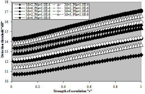
After formulating the processor performance for M- correlated sweeps, it is of great importance to provide a variety of numerical results for the performance of the fixed- threshold detector in order to take an idea about the role that each parameter can play in controlling the behavior of the detection scheme against the environmental changes. Since the choice of the detection threshold represents the principal parameter of the processor performance, Fig.(16) depicts the variation of this threshold with the selected rate of false alarm for several values of the sweep-to-sweep correlation coefficient when the radar receiver integrates 2 and 4 consecutive pulses to formulate the background level against which the target return is compared to decide its presence or absence. For lower rate of false alarm, the required threshold to achieve this rate becomes of high level. However, this level varies as the correlation between consecutive sweeps changes. It attains its maximum value when the successive sweeps are fully correlated (ρ=1) and decreases as the correlation coefficient decreases till it attains its minimum value in the case where the consecutive sweeps become uncorrelated (ρ=0). As the false alarm rate increases, the different curves approach each other till they become coincide at a false alarm probability of 0.316, for two consecutive sweeps, beyond which the reverse behavior is noticed. It is well-known that as the correlation between consecutive sweeps increases, the effective value of the noise level decreases and this in turn leads to increase the detection threshold for the required rate of false alarm to be held constant. On the other hand, as M increases, the threshold increases, as we have previously explained in Fig.(2), given that the correlation level as well as the false alarm rate rest unchanged. To illustrate the effect of correlation on the determination of the detection threshold, Fig.(17) shows the changing of the threshold (in dB) with the sweep-to-sweep correlation coefficient for various values of the required level of false alarm as well as the number of integrated correlated pulses. The behavior of the curves of this figure indicates that there is a negligible increment in the detection threshold till the correlation level of the consecutive sweeps reaches 12% after which it increases, in approximately a linear manner. The rate of increasing is nearly the same, for fixed number of integrated pulses, whether the required rate of false alarm is low or high. For fixed level of false alarm, on the other hand, the rate of increasing varies as M increases. There is a small incremental change in the rate of increasing of the detection threshold as M varies from 2 to 4.Once the detection threshold is constructed, the variation of the probability of detection as a function of the signal strength is taken as a figure of merit that distinguishes one processor over the other. Fig.(18) displays these characteristics for the underlined scheme when M correlated sweeps are integrated to represent the source of data that supplies the obtained numerical results. As predicted, increasing the correlation between the consecutive sweeps degrades the processor performance. This degradation is of noticeable value in the range 3-23dB in the case of M=2, while it extends from 1dB to 21dB in the case of M=4. The worst case is obtained when the consecutive sweeps are fully correlated. As we have shown from the results of Figs.(16-17), increasing ρ yields higher values for the detection threshold and in the same time decreases the signal strength.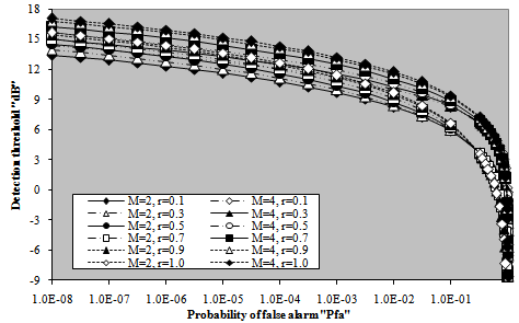 | Figure 16. M-correlated sweeps detection threshold as a function of the false alarm rate for different values of sweep-to-sweep correlation coefficient |
 | Figure 17. M-correlated sweeps detection threshold as a function of consecutive pulses correlation coefficient of fixed-threshold processor |
Consequently, the achieved detection level becomes lowered. For the same level of signal strength, the detection performance improves as either M increases or ρ decreases. Fig.(19) confirms this extracted remark. It presents the same processor detection performance in another manner. The obtained value of detection probability is plotted against the sweep-to-sweep correlation coefficient for different values of signal strength for the case where there are two and four integrated sweeps, given that the required rate of false alarm is kept at 10-6. It is obvious from the behavior of the candidates of the underlined figure that the processor performance degrades as the correlation between the consecutive sweeps becomes stronger. The rate of degradation depends on the signal strength. It decreases as the strength of the signal increases. For higher signal levels (α=25dB), the degradation rate becomes of negligible value and the detection performance seems unchanged with the strength of correlation between successive sweeps. Finally, as an excellent trend for measuring the detection performance of any processing scheme is to calculate the required SNR to achieve pre-assigned values for the level of detection and the rate of false alarm. Fig.(20) illustrates the variation of the required signal strength as a function of the level of correlation between consecutive sweeps. The curves of this figure are parametric in M and the demand rate of false alarm. The needed level of detection is taken as 90% throughout the entire candidates of the figure. The demand rate of false alarm is chosen to be varied from 10-4 to 10-8. The shown results demonstrate that as the correlation strength increases, more signal strengths are required to attain a given level of detection. In other words, as the consecutive sweeps become strongly correlated, the grade of degradation in the processor performance increases in such a way that it has its worst behavior when the successive sweeps are fully correlated. Additionally, as the required rate of false alarm decreases, the necessary signal strength to respond the needed level of detection increases owing to the higher values of the demanded threshold to achieve this rate. For weak correlation, the computed SNR seems approximately constant. As the correlation becomes stronger, on the other hand, the evaluated signal strength increases, in a nearly linear manner, till it reaches its peak value at ρ equals unity. Moreover, as the number of integrated pulses increases, the resulting signal level decreases, given that the required values for the rate of false alarm and the level of detection are held unchanged.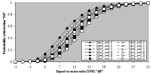 | Figure 18. M-correlated sweeps detection performance of fixed- threshold detector for false alarm rate of 1.0E-6 |
 | Figure 19. M-correlated sweeps detection performance against the strength of correlation between consecutive sweeps of fixed-threshold scheme |
 | Figure 20. M-correlated sweeps required SNR, to achieve different operating points, against the strength of correlation between consecutive pulses of fixed-threshold detector |
5. Conclusions
The detection performance of an optimum radar receiver, which postdetection integrates M pulses from fluctuating targets; obeying χ2 distribution with K degrees of freedom in their fluctuation, is analyzed. The well-known Swerling cases I-IV corresponds to K=1, M, 2, and 2M, respectively. At the limiting case (K=∞), the processor performance attains its maximum response and the radar target becomes stationary (nonflucruating). From the fluctuation point of view, target amplitudes are Rayleigh distributed for SWI and SWII models, while they are χ2 distributed for SWIII and SWIV. From the strength of correlation point of view, on the other hand, the correlation coefficient between the two consecutive echoes in the dwell-time is equal to unity for SWI and SWIII models, while it is zero for SWII and SWIV fluctuation cases. Moreover, we have analyzed the performance of the fixed-threshold processor for partial signal correlation in the situation where the primary target is assumed to be fluctuating in accordance with χ2 model with two and four degrees of freedom. Our analysis is based on evaluating the moment generating function of the incoming signal, which is immersed in clutter. A closed form expression for the false alarm and detection probabilities is used to develop a complete set of performance curves including detection probability against the strength of the primary target, required SNR to achieve a prescribed value of false alarm rate and level of detection. As expected, the detection performance of the underlined scheme for partially correlated χ2 targets with two degrees of freedom is greater than that of SWI case and less than that for SWII target's model. On the other hand, the fixed-threshold processor performance, for partially correlated χ2 targets with four degrees of freedom, is higher than that for SWIII case and lower than that for SWIV target fluctuation model. Therefore, to estimate the performance for partially correlated pulses, interpolation between the results for completely correlated and completely decorrelated conditions can be used as an approximation. In any one of the fluctuating families, more per pulse signal-to-noise ratio is required to achieve a prescribed probability of detection as the signal correlation increases from zero to unity. In addition, we have given a detailed evaluation of the detection performance of the fixed- threshold scheme when the supplemented data is fitted to it through a moving target indicator. Since the output sequence of this device is correlated, even if its input sequence is not, the radar receiver is supplemented by a video integrator that incoherently integrates M-pulses. The purpose of the integrator is to enhance the detection probability of a periodic sequence of pulses. The numerical results provide an important insight into the effect of the system’s parameters on its performance. As a final conclusion, the detection performance of fixed-threshold detector is related to the target model, the number of noncoherently or incoherently integrated pulses, and the average power of the target.
References
| [1] | Meyer, D. P. & Meyer, H. A., “Radar target detection”, Academic Press, INC. 1973 |
| [2] | El Mashade, M. B., “M-sweeps detection analysis of cell- averaging CFAR processors in multiple target situations”, IEE Radar, Sonar Navig., Vol.141, No.2, (April 1994), pp. 103-108 |
| [3] | El Mashade, M. B., “Performance analysis of OS family of CFAR schemes with incoherent integration of M-pulses in the presence of interferers”, IEE Proc.-Radar, Sonar Navig., Vol.145, No.3, (June 1998), pp. 181-190 |
| [4] | Mahafza, B. R., "Radar systems Analysis and design using Matlab", Chapman & Hall/CRC, 2000 |
| [5] | El Mashade, M. B., “M-correlated sweeps performance analysis of Mean-Level CFAR processors in multiple target environments”, IEEE Transactions Aerospace and Electronic Systems, AES-38, No. 2, (April 2002), pp. 354-366 |
| [6] | Osche, G. R., “Optical detection theory for laser applications”, John Wiley & Sons, INC., Publication, 2002 |
| [7] | El Mashade, M. B., “Target multiplicity performance analysis of radar CFAR detection techniques for partially correlated chi-square targets”, Int. J. Electron. Commun., (AEÜ), Vol.56, No.2, (April 2002), pp.84-98 |
| [8] | El Mashade, M. B., "Exact performance analysis of OS modified versions with noncoherent integration in nonideal situations", Journal of the Franklin Institute, Vol. 342, (2005), pp.521-550 |
| [9] | El Mashade, M. B., "Performance Comparison of a Linearly Combined Ordered-Statistic Detectors under Postdetection Integration and Nonhomogeneous Situations", Journal of Electronics (China), Vol.23, No.5,(September 2006), pp. 698-707 |
| [10] | El Mashade, M. B., “Exact performance analysis of the generalized trimmed-mean CFAR scheme for moderately fluctuating radar targets”, Accepted for publication in Signal Processing “ELSEVIER”. |
| [11] | El Mashade, M. B., “Target multiplicity exact performance analysis of ordered-statistic based algorithms for partially correlated chi-square targets”, Accepted for Publication in IEE Proc.-Radar, Sonar Navig |
| [12] | El Mashade, M. B., “CFAR detection of partially correlated chi-square targets in target multiplicity environments”, Accepted for Publication in Int. J. Electron. Commun. (AEÜ) |
| [13] | El Mashade, M. B., "Analysis of CFAR detection of fluctuating targets", Progress in Electromagnetic Research C. Vol. 2, pp.65-94, 2008 |
| [14] | El Mashade, M. B., "Performance analysis of OS structure of CFAR detectors in fluctuating target environments", Progress in Electromagnetic Research C. Vol. 2, pp.127-158, 2008 |
 Abstract
 Reference
 Full-Text PDF
 Full-Text HTML