-
Paper Information
- Next Paper
- Previous Paper
- Paper Submission
-
Journal Information
- About This Journal
- Editorial Board
- Current Issue
- Archive
- Author Guidelines
- Contact Us
Electrical and Electronic Engineering
p-ISSN: 2162-9455 e-ISSN: 2162-8459
2011; 1(2): 79-84
doi: 10.5923/j.eee.20110102.13
Analysis of Performance and Implementation Complexity of Array Processing in Anti-Jamming GNSS Receivers
 Abstract
 Reference
 Full-Text PDF
 Full-Text HTML
Chung-Liang Chang , Bo-Han Wu
Department of Biomechatronics Engineering, National Pingtung University of Science and Technology,
Correspondence to: Chung-Liang Chang , Department of Biomechatronics Engineering, National Pingtung University of Science and Technology,.
| Email: |  |
Copyright © 2012 Scientific & Academic Publishing. All Rights Reserved.
This paper investigates the existing spatial-temporal interference suppression methods which attempt to mitigate interference before the GNSS receiver performs correlation. These methods comprise non-blind signal processing techniques and blind signal processing techniques by using the antenna array. Also, an extensive comparison of these techniques for GNSS is established, which is evaluated from the view of convergence rate, numerical stability, computational loads, and realization complexity. The research offers a foundation of the spatial-temporal adaptive processing (STAP) practical realization and the design for new processors.
Keywords: STAP, GNSS, Anti-Jam Techniques
Cite this paper: Chung-Liang Chang , Bo-Han Wu , "Analysis of Performance and Implementation Complexity of Array Processing in Anti-Jamming GNSS Receivers", Electrical and Electronic Engineering, Vol. 1 No. 2, 2011, pp. 79-84. doi: 10.5923/j.eee.20110102.13.
Article Outline
1. Introduction
- In recent years, spatial-temporal adaptive processing (STAP) is a well- known technique that has been proposed to remove narrowband interference and eliminate broadband interferences[1-5]. Most of these algorithms may be categorized into three classes according to whether a training signal is used or not. One class of these algorithms is the non-blind adaptive algorithm in which a training signal is used to adjust the array weight vector. Another technique is to use a blind adaptive algorithm which does not require a training signal. Still another is semi-blind adaptive algorithm in which the desired signal information can be obtained by inertia navigation system.Generally, it takes three steps to employ STAP so as to deal with interference mitigation. The first step is to estimate the covariance matrix of input signal. The second step is to utilize adaptive algorithm in order to obtain weight vector. The last step is to output signal through the addition acquired by weighting the measurement data. Each algorithm outperforms others in a specific way. For example, some are better in performance. However, they are higher in implementation complexity and longer in computation time, which makes it difficult in real time processing and hardware implementation. As a result, in addition to taking performance into consideration, we must also consider hardware implementation complexity and computation cost. Besides, huge adoption of multiplications/additions also increases cost. Thus, proper adjustment in algorithm form such as reducedrank and possible implementation can upgrade system performance to a certain degree. This paper focuses on analyses and evaluation of the performance of commonly used STAP techniques in order to further understand the benefits and drawbacks and provide evaluation reference in hardware implementation.The remainder of this paper is organized as follows. Section 2 gives a description of GPS signal model. It also briefly reviews various types of STAP algorithm. The comparison of STAP requirement and implementation complexity is given in Section 3. Finally, a short summary follows in Section 4.
2. Stap Overview
- In this section we analyze an adaptive spatial-temporal processing for GPS interference mitigation processing. The design criterion of adaptive antenna algorithm can be imposed at spatial domain or temporal domain. One class of these algorithms is the non-blind adaptive algorithm in which a training signal is used to adjust the array weight vector. For example, it contains least-mean squares method (LMS)[6], sample matrix inversion method (SMI)[7], recursive least-squares (RLS) method[8], minimum variance distortionless response (MVDR) method[9,10], and multistage nested wiener filter (MSNWF)[11], etc. Another technique is to use a blind adaptive algorithm which does not require a training signal. Namely, it consists of power minimization (PM) method[12], and Reduced-rank PM approach, etc. These techniques are employed to dynamically adjust antenna array pattern response to further reduce the power of interfering signal sources. In this section, according to the results of study, we give the general spatial-temporal signal model for GPS interference mitigation. The spatial-temporal signal model at the
 sample of
  antenna element can be described as
  matrix:
 | (1) |
 ,
,  is number of tap of each antenna,
  denotes the conventional transpose,
  ;
;  ,
,  ,
,  has the same structure as
  ,
,  is the total number of interfering signals,
  denotes the Kronecker product operator, and
  is the sampling rate;
  is zero-mean, temporal and spatially white with variance
  .
.  and
and  denote the
  steering vector with respect to GPS satellite and
  interfering source, respectively. The spatial-temporal weight vector can be described as
  | (2) |
 and
and  are
are  column vectors. In the following, several STAP methods are described.
 2.1. LMS Algorithm
 | (3) |
 is the expectation value,
  is the delay of the training signal selected to output the best performance, and
  denotes a Euclidean norm of a vector. Because the covariance matrix,
  , and the cross-correlation vector,
  , are not known prior to processing, one uses their instantaneous estimates, as
 | (4) |
 | (5) |
 | (6) |
 a gain constant to control convergence. Due to the extreme simplicity of this algorithm, it may also be implemented by analog means. Nevertheless, its convergence relies on the eigenvalue spread of
  , and in practical situations it is often too slow.
2.2. SMI Algorithm
- This algorithm overcomes the convergence problem of the LMS algorithm. By solving this optimum question, we can find
 | (7) |
 and the cross- correlation matrix
  , by time-averaging from the block of input data. The estimate of the covariance matrix
  is given by:
 | (8) |
 | (9) |
 denotes the
  input signal vector. From Eq. (8) and (9), it is possible to compute several (
 ) LS-solution for a single snapshot
  . These solutions can be combined (after they all are computed) by adding them together. In this method, the correlation matrix and weighting vector computed with respect to the previous spatial-temporal block is utilized. It is called time coherent block adaptive beamforming and the new weighting vector is updated in accordance with
  | (10) |
 . Note that the processor is also repeated for each GPS satellite to calculate user’s position and requires attitude information.
2.3. RLS Algorithm
- A method by estimating both
 and
and  using the weighted sum is employed to overcome not only the convergence limitations of the LMS algorithm but also the numerical and calibration issues of the SMI algorithm.
 | (11) |
 | (12) |
 ,
,  , puts more emphasis on the most recent samples than the older data. After some manipulation, the weight vector may be updated by
  | (13) |
 given by
 | (14) |
2.4. MVDR Algorithm
- We assume that the direction of signal of interest is known. The MVDR technique is used to minimize the output noise variance in accordance with placing constraints. The following MVDR with
 linear constraints:
 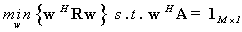 | (15) |
 is as depicted in Eq (1). The minimization can be solved using the Lagrange multiplier techniques and the spatial-temporal MVDR optimal solution is given by the following expression:
 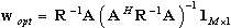 | (16) |
 , is known, and is referred to as an optimal beamformer. However, the existence of steering vector error worsens the performance of the approach. In practice the covariance matrix is not known but rather must be estimated using training data.
2.5. PM Algorithm
- Because the received GPS signal power is well below the thermal noise floor, we can simply constrain the weight on the first tap of reference antenna 1, and then minimize the output power, namely:
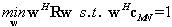 | (17) |
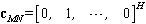 is the
  vector. The weights for the auxiliary antennas are determined when those which drive the output power of the beamformer are down to the noise floor as possible. Thus, using the method of Lagrange multipliers, the solution to (17) is
 | (18) |
2.6. Reduced-Rank PM Algorithm
- Owing to the large dimensionality of the spatial-temporal covariance matrix and weight vector, STAP techniques will result in a larger computational burden and convergence slowly. Consequently, the reduced-dimension method has been proposed recently. Reduced-dimension methods are mainly adopted so as to constraint weight vector to lie in a lower dimensional subspace by the transformation matrix
 , namely let:
 | (19) |
 | (20) |
 | (21) |
 is Hermitian-symmetric with
  dimension matrix, which is less than the one of
  , it leads to lower computational complexity and rapid convergence. The reduced dimension transformation matrix
  can be found by techniques such as the cross-spectral (CS) metric or principal-components (PC).
2.7. MSNWF Technique
- Dr. Zoltowski proposed a reduced-dimension STAP technique based on MSNWF. It is illustrated that the MSNWF does not require computing the inversion of
 , thereby reducing computational complexity. The MSWF algorithm is summarized below. The interpretation of the “desired” signal
  varies amongst the different type of spatial-temporal processors. • Initialization:
  and
and  • Forward Recursion: for
  :step 1. Compute the weights vector
 step 2. Compute the intermediate vector
 step 3. Update the output vector
 • Backward Recursion: for
  with
with  step 1. Compute and update the single weight vector
 It is crucial to observe that all operations of the MSNWF involve complex vector-vector products, not complex matrix-vector products (for the single space-time weight constraint), there by indicating computational complexity
  per snapshot. The MSNWF algorithm can reduce computational complexity and improve the speed of convergence compared with CS metric or PC.
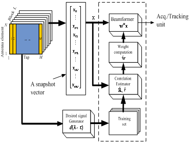 | Figure 1. Illustration of the STAP procedures |
3. System Computation Requirement and Comparison
- The computation requirements in STAP techniques arise from the need to cancel unwanted interference and improve the signal-to-noise ratio. Figure 1 shows the STAP typically performed in one coherent processing interval, which consist of
 blocks,
  delay time tap, and
  antenna elements. The resulting training set is used to compute the weights that are applied to the entire data matrix. The beamforming operation is a matrix-vector multiplication,
  , where
  is the output data in that beam. In general, there are two computational criteria that a practical implementation should ideally possess to achieve sufficient interference suppression: a rapid convergence rate (i.e., sample support size) to reduce nonhomogenous samples that contribute for the interference covariance estimation and a low computational complexity for real-time processing[13, 14]. For convenience, the comparison of various adaptive algorithms in terms of numerical stability and computation efficiency are given in Table 1. It is known that the family of the “Fast” least squares has serious numerical instability in limited precision environment. For example, the steady error of algorithm in SMI, RLS is small but it takes a long time to calculate. MSNWF is more efficient in calculation time due to its adoption of reduced rank and Multi-stage. SMI is rapid in convergence rate; however, it is subject to numeric instability due to the matrix inversion with finite-precision representation of the matrix entries.LMS is simple in calculation and thus easier in hardware implementation. In contrast, SMI, RLS and MVDR are more complicated in hardware implementation owing to its requirement of input signal covariance matrix. Later on, MSNWF is proposed to reduce complexity in hardware implementation. However, besides matrix, inside the structure of these methods are major differences, which also decide the implementation complexity of processors. However, it is necessary to compute a gain vector in RLS, which requires a large amount of computational cost. On the other hand, the hardware implementation complexity in both PM and Reduced-rank PM is greatly reduced because they merely deal with single antenna weight vector. The computational complexity is reduced in MSNWF because it employs reduced rank techniques and does not require computing matrix inversion with the perquisite of satellite direction known for available utility.
|
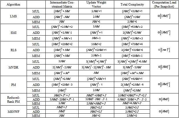
- If the computation load is too high when utilizing STAP in real time, there is not only difficulty in system implementation but also loss of real time on line. Table 2 illustrates multiplications, additions as well as memory required in single measurement data through different STAP algorithms.Take SMI for example. We consider inverse matrix operator, which requires multiplications
 and additions
  . The computational load needed in adjusting the weight value requires multiplications
  and additions
  , which calls for multiplications
  and additions
  in total computation complexity. In addition, it requires at least memory
  unit and total computational load
  unit. If the dimension of matrix is too high in SMI, the computational load will be too large to be utilized in hardware implementation. When we compare LMS and RLS, LMS is simpler in hardware complexity, which is due to the calculation of gain vector factor in RLS.(see Table 2) It takes large computation load in MVDR because the weight vector of each antenna has to be adjusted in this algorithm. In contrast, the weight vector of only single antenna has to be adjusted in PM. Therefore, MVDR is higher in hardware implementation complexity. The computational time in Reduced-rank PM and MSNWF is far shorter than that in other algorithms, which is due to the fact that they do not require inverse matrix value and in turn, the computational time is much shorter.
4. Conclusions
- This paper makes comparisons and analyses from typical STAP performance, mainly from not only computation load, multiplications and additions required in algorithm but also realization complexity. The research analysis is derived as follows: Firstly, MSNWF is best in performance. This approach employs reduced rank to proceed; therefore, its complexity is the lowest in hardware implementation. However, this algorithm is also limited because the information of satellite signal direction should be required in advance. Secondly, LMS is easier in hardware implementation. However, because its steady state error is larger, its performance is worse and not practical in general condition.Thirdly, RLS and SMI are only second to MSNWF in performance. Nevertheless, their computation load is the highest. Under the condition of heavy interference, the adoption of multiple antennas and tap number makes them (RLS and SMI) higher in hardware implementation complexity than other algorithms. As a result, they are not practical in use. Fourthly, PM and Reduced-rank PM are medium in performance. These two approaches do not require the information of satellite direction. Moreover, because Reduced-rank PM utilizes reduced rank, the time needed in computation load is greatly reduced, which makes it rather convenient in hardware implementation. We can acquire transformation matrix by such methods as CS or PC. However, both methods are quite a computational burden since it is necessary to produce eigenvectors of covariance matrix before finding transformation matrix.Lastly, MVDR is more stable in performance without beamforming. Though its hardware implementation complexity is higher, it can be a good choice when the antenna numbers are fewer. From the above analyses, we can distinguish the benefits and drawbacks of STAP performance and in turn provide a reference for future hardware implementation and development of new processors. To sum up, a processor can not be generally and broadly defined as superior or inferior. Nevertheless, under certain condition and requirement, it is possible to evaluate the overall performance.
ACKNOWLEDGEMENTS
- The author would like to thank the National Science Council of R.O.C. for their support of this work under NSC 100-2221-E-020 -027.
References
| [1] | R. L. Fante, and J. J. Vaccaro, “Cancellation of jammers and jammer multipath in a GPS receiver,” IEEE AES System Magazine, vol. 13, pp. 25–28, November 1998 |
| [2] | R. L. Fante and J. J. Vaccaro, “Wideband cancellation of interference in a GPS receiver array,” IEEE Trans. on Aerospace and Electronic Systems, vol. 36, no. 2, pp. 549-564, April 2000 |
| [3] | X. Ping, J. M. Michael, and N. B. Stella, “Spatial and temporal processing for global navigation satellite system: The GPS receiver paradigm,” IEEE Trans. on Aerospace and Electronic Systems, vol. 39, no. 4, pp.1471-1484, 2003 |
| [4] | G. Hatke, “Adaptive array processing for wideband nulling in GPS system,” in Proceedings of the 32nd Asilomar Conference on Signals, Systems and Computers, vol. 2, pp. 1332-1336, 1998 |
| [5] | C. L. Chang, J. C. Juang, ‘Analysis of spatial and temporal adaptive processing for GNSS interference mitigation,’ Proc. of International Symposium on IAIN/GNSS, ICC Jeju, Korea, Oct. 2006 |
| [6] | S. Hyakin, Adaptive Filter Theory, 3rd Ed., Prentice Hall, Englewood Cliffs, 1996 |
| [7] | J. Litva and T. K.-Y. Lo., Digital Beamforming in Wireless Communications, Artech House, Boston, 1996 |
| [8] | Z. Tian, K. L. Bell, H. L. Van Trees, “A recursive least squares implementation for LCMP beamforming Under Quadratic Constraint,” IEEE Trans. on Signal Processing, vol. 49, no. 6, June, 2001 |
| [9] | J. Li, P. Stoica, and Z. Wang, “On robust capon beamforming and diagonal loading,” IEEE Transactions on Signal Processing, vol. 51, pp. 1702-1715, July 2003 |
| [10] | C. Tang, K. Liu, S. Tretter, “Optimal weight extraction for adaptive beamforming using systolic arrays,” IEEE Trans. on Aerospace and Electronic System, vol. 30, No. 2, April 1994 |
| [11] | W. L. Myrick, J. S. Goldstein, and M. D. Zoltowski, “Low complexity anti-jam space-time processing for GPS,” Proceedings of the 2001 IEEE International Conference on Acoustics, Speech, and Signal Processing, vol. 4, pp. 1332- 1336, 2001 |
| [12] | Y. T. J. Morton, L. L. Liou, D. M. Lin, J. B. Y. Tsui, and Q. Zhou, “Interference cancellation using power minimization and self-coherence properties of GPS signals,” in Proceedings ION GNSS Conference, Long Beach, CA, 2004 |
| [13] | R. Blazquez, J. M. Blas, and J. I. Alonso, “Implementation of adaptive algorithms for array processing in real time application to low cost GPS receivers,” IEEE 49th Vehicular Technology Conference, vol. 1, pp. 463-467, May 1999 |
| [14] | D. C. Ricks and J. S. Goldstein, “Efficient architectures for implementing adaptive algorithms,” in Proceedings of the 2000 Antenna Applications Symposium, pp. 29-41, Allerton Park, Monticello, Illinois, September 20-22, 2000 |