Marcel Stamate , Petrica Taras, Virgiliu Firetean
EPM_NM Laboratory, Faculty of Electrical Engineering, University POLITEHNICA of Bucharest, Bucharest, 060042, Romania
Correspondence to: Marcel Stamate , EPM_NM Laboratory, Faculty of Electrical Engineering, University POLITEHNICA of Bucharest, Bucharest, 060042, Romania.
| Email: |  |
Copyright © 2012 Scientific & Academic Publishing. All Rights Reserved.
Abstract
The paper studies the possibility of measuring active power in induction heating applications by using the proximate electromagnetic field to extract information about the power factor of the device. The method consists of using an external coil sensor placed in the device proximity. Two induction heating systems are studied. The first application concerns a helical inductor and a lateral sensor and the second, a spiral inductor with an underneath placed sensor. Different positions of the coil sensor are considered in order to search for the position for which the phase of the output sensor voltage is equal with the shift phase between the voltage and the current with respect the inductor terminals. The investigation is carried out by using 2D finite element models.
Keywords:
active power measurement, induction heating, proximate magnetic field, finite element computation
Cite this paper:
Marcel Stamate , Petrica Taras, Virgiliu Firetean , "Non-Intrusive Measurement of Induction Heating Systems Active Power through the Proximate Magnetic Field", Electrical and Electronic Engineering, Vol. 1 No. 1, 2011, pp. 1-7. doi: 10.5923/j.eee.20110101.01.
1. Introduction
Active power absorbed by an electric system is the average of the instantaneous power u(t)i(t):  | (1) |
If the voltage u(t) and the current i(t) with respect the supply terminals are sinusoidal, then the active power is:  | (2) |
A precise enough measurement of active power at the terminals of an inductor coil means determining the voltage U, the current I and the phase shift φ with relatively small errors. High errors of active power measurement occur when the phase shift is close to 90°. The relative error is determined with the following relation:  | (3) |
The last term in (3) introduces very high errors in the power measurement, even when the angle φ is determined with a 1 % precision. It is possible to measure with a good precision the phase shift φ by using a non-intrusive approach. The solution consists in using an external coil sensor placed in the inductor proximity. Based on the finite element model of the system, where the imposed current in the inductor has the phase zero, different positions of the sensor are considered in order to search for the particular ones where the phase of the sensor output voltage is the same with the phase of the inductor supply voltage.Two induction heating configurations were considered: a helical inductor around a cylindrical charge and a spiral inductor for flat plates heating. Different materials of the heated charge where considered in order to obtain a relatively large range of the shift phase between the inductor voltage and current.
2. Finite element models
The finite element models involved in the study are steady state AC magnetic type of applications. The inductor power supply frequency is 5 kHz. Both models reflect 2D axisymmetric applications.Figure 1a contains the geometry of the first model. The studied inductor is a longitudinal flux type (Figure 2).It was possible to take into account only a quarter of the device geometry. The mesh grid is shown in the Figure 1b. A high mesh density is given on the three turns of the inductor and on the charge surface Charge regions which are solid conductors regions. In this way the skin effect can be considered more precise. The Inductor region turns are physically implemented as massive hollow rectangular shape section copper conductor. The inductor is water cooled.The study can be conducted with or without the Charge regions which is also, if present, a solid conductor. Different materials are tested for the Charge region. The materials used are copper, aluminium and various steels with values for the magnetic relative permeability (1, 10, 100, 1000). Also a steel with a nonlinear magnetic properties (initial magnetic relative permeability is 1500 and the saturation magnetization is 1.5 T) is used as charge material. 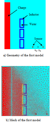 | Figure 1. The computation domain and mesh grid of the first model |
The Sensor region, placed close to the inductor, is a stranded coil conductor (50 turns) connected to a 1 MΩ resistor which models a voltmeter connected to the coil. The coil Sensor can be positioned in a various points of the computation domain in order to retrieve the information regarding the phase.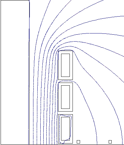 | Figure 2. Isoflux lines in the longitudinal inductor |
Boundary conditions take into account the existing physical symmetries on the Ox and Oy boundary axes. The magnetic field is imposed as tangential to the Oy axis and normal to the Ox axis.The second model is presented in Figure 3a. Its mesh is given in Figure 3b.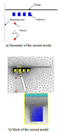 | Figure 3. The computation domain and mesh grid of the second model |
Computation domain contains the same regions and their associated physical properties as the previous model albeit with a different geometric shape.The second model inductor is a transversal type (Figure 4).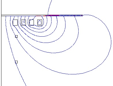 | Figure 4. Isoflux lines in the transversal inductor |
The addition of a charge near the inductor coil is also investigated in terms of sensor measurements. Different positions of the sensor are tested in order to search for a desired position in which the studied phases are similar.
3. Helical coil finite element model results
This investigation involves repeated studies for different position of the sensor coil. The sensor coil center point (xc, yc) is varied in the [65 … 200 mm] x [2 … 64 mm] planar interval with respect to the coordinate system origin (Figure 5).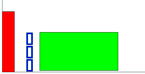 | Figure 5. Search area of positions of the center of sensor (xc,yc) |
This interval covers the area from the lateral of the device with a precision of 10 x 8 = 80 points. The main results of the finite element models are the phase isoline, i.e. the geometrical places of the coil sensor center in which the phase of the induced coil voltage is equal with the voltage phase on the inductor. The number associated to the isoline represents the common value of the voltage phase on inductor and sensor coil.When the charge cylinder is not present, the isoline of the same value as the inductor voltage phase is given in Figure 6. The value of the inductor voltage phase is written in every figure close by the curve. For this case this is 88.2 degree.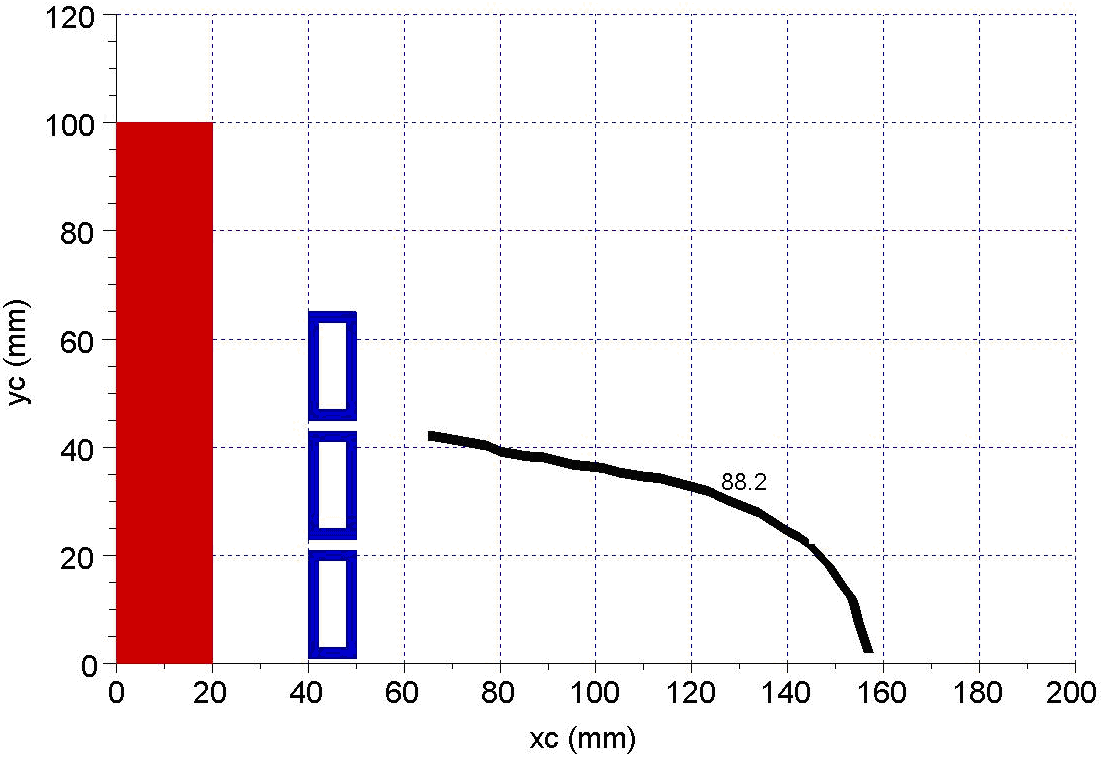 | Figure 6. Phase dependence on (xc,yc) position for no change |
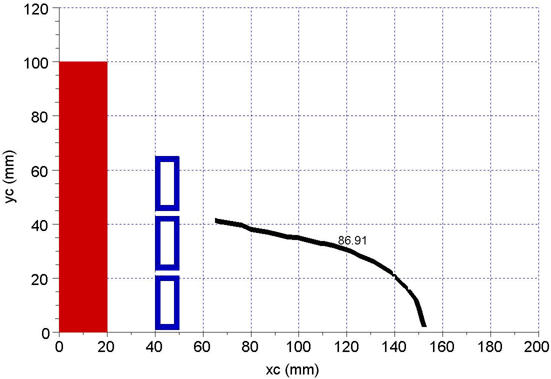
Using a copper cylinder as charge, the isoline on the studied interval is represented in Figure 7. For aluminium as charge the contour line is shown in Figure 8.The superposition of the isolines from Figures 6 - 8 shows that the aluminium and copper charge cylinders do not modify too much the magnetic field configuration (Figure 9) with respect to the “no charge” case.  | Figure 7. Phase dependence on (xc,yc) position for copper |
 | Figure 8. Phase dependence on (xc,yc) position for aluminium |
The copper and aluminium isolines, in Figure 9, are practically overlapped while the “no charge” isoline is close to the other two.Next, the study is conducted for steel like class of materials with the permeability ranging from 1 to 1000 but with the same value of the electric resistivity.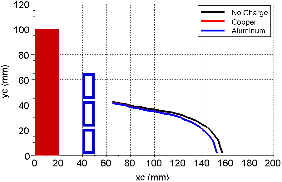 | Figure 9. The no charge, copper and aluminium isolines comparison |
Figure 10 contains the phase isoline for a charge cylinder made of nonmagnetic steel. The isoline is close, in shape and position, to the previous three.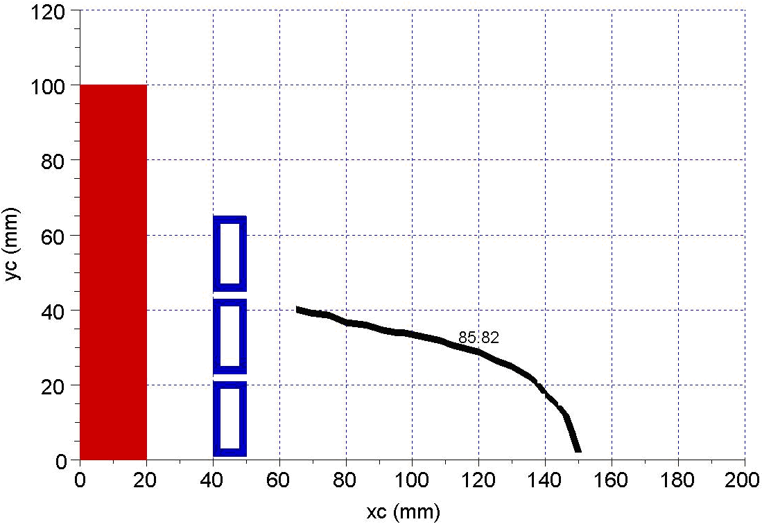 | Figure 10. Phase dependence on (xc,yc) position for non-magnetic steel |
In Figure 11 a magnetic (μr = 10) steel cylinder is used as charge. The surrounding magnetic field configuration is affected due to higher power absorption of the cylinder charge.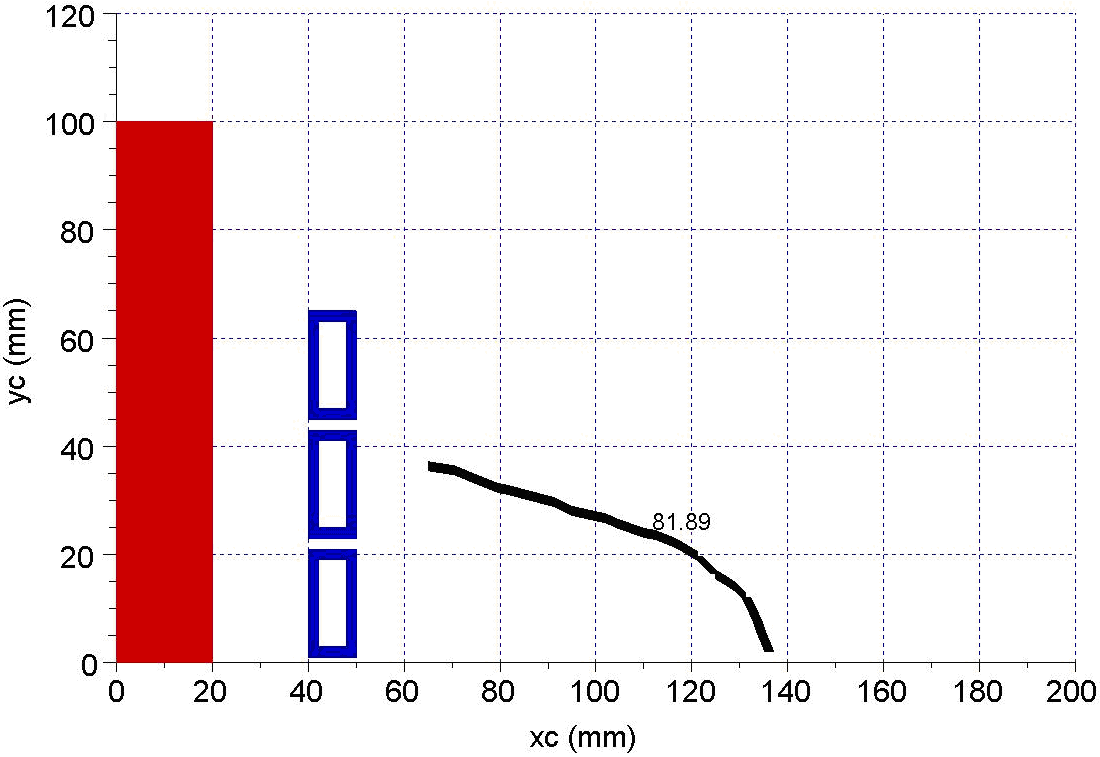 | Figure 11. Phase dependence on (xc,yc) position for μr = 10 magnetic steel |
Figures 12 and 13 contain the results for a steel charge with permeability of 100, respectively 1000.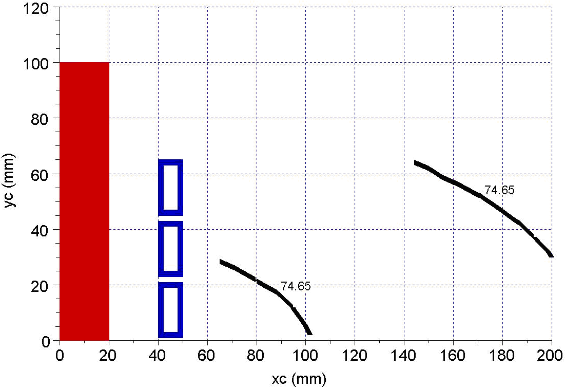 | Figure 12. Phase dependence on (xc,yc) position for μr = 100 magnetic steel as charge material |
 | Figure 13. Phase dependence on (xc,yc) position for μr = 1000 magnetic steel as charge material |
The general tendency of the phase isoline is to get closer to the inductor as the permeability of the charge steel increases.Table 1 contains a comparison between the active power values absorbed by different charges. The active power induced in charge increases gradually with the permeability for charges made of steel.| Table 1. Comparison between actives powers induced in charge [kW] |
| | No charge | Alu- minium | Copper | Steel | | | | | µr=1 | µr=10 | µr=102 | µr=103 | | 0 | 0.28 | 0.21 | 0.63 | 2.03 | 5.75 | 13.2 |
|
|
Figure 14 shows the geometrical place for positions of the center of the sensor for that the value of voltage phase measured is the same with value of the voltage phase on terminals of the induction heating system.It is easy to observe that, even for steel with a nonlinear permeability, are some positions where the sensor can estimate precisely the voltage phase. These results show that for every material used as charge exist some positions for which the voltage phase of the inductor is determined.Therefore, is possible to build a measurement system to measure the active power absorbed by an induction heating system based on the proximate magnetic flux. This sensor coil can accurately estimate the voltage phase on the inductor and then with relation (2) the active power is known.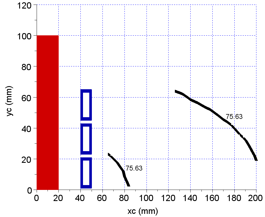 | Figure 14. Phase dependence on (xc,yc) position for magnetic steel with nonlinear permeability as charge material |
4. Spiral coil finite element model results
The second finite element model is a cooking plate application. The Charge region is actually the pot bottom and can be made of copper or aluminium for an increased efficiency. Due to this fact, the Charge region material, when present, must be either copper or aluminium. However, steel is used also as charge in order to investigate the inductor magnetic field configuration for higher permeability.In the second finite element model the interval of study is [15 … 90] x [-60 … -25 mm] (Figure 15). The grid covering this interval has 16 x 8 = 128 points, meaning that a total of 128 models are solved in order to obtain the required phase variation. The study interval is placed under the device due to the fact that the magnetic field is stronger there.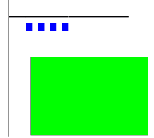 | Figure 15. Position of the center of sensor marked in the second model |
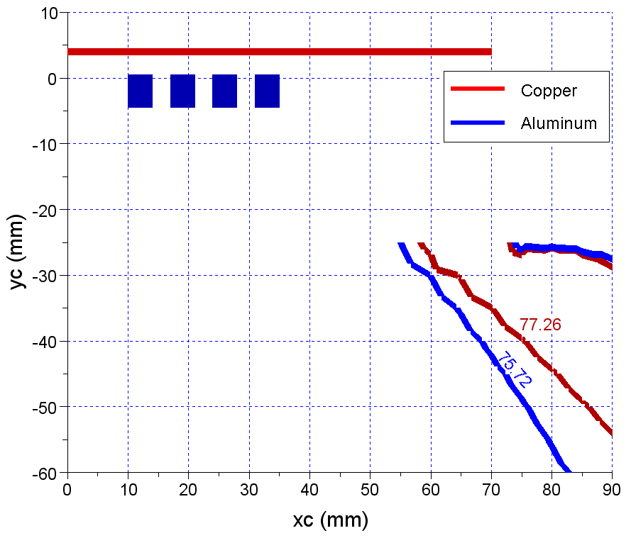
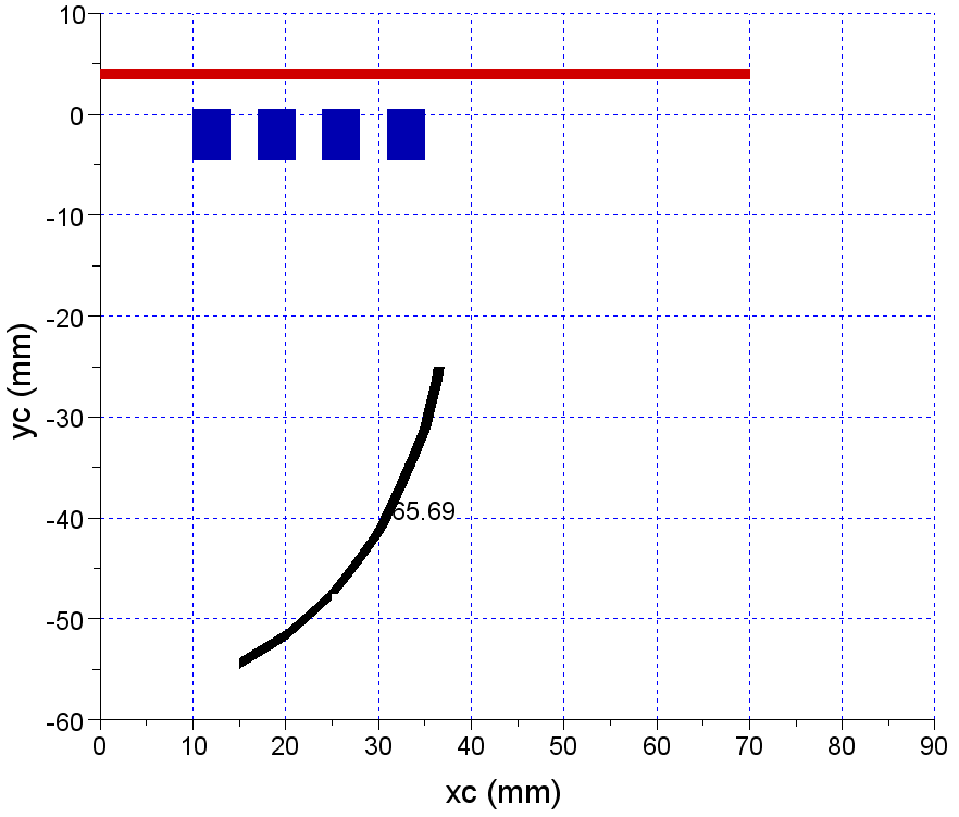
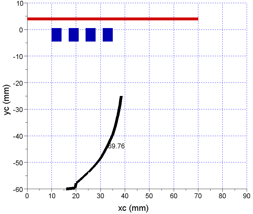
When the charge is missing, the sensor can not find any isoline corresponding to the inductor voltage phase. When the cooking pot is made of aluminium, the isoline from Figure 16 is obtained.If the charge is made of copper, the contour line from Figure 17 is obtained.There are however similarities between Figs 16 and 17. Figure 18 contains the superposition of the “al” and “cu” isolines. The contour lines in question overlap partially. 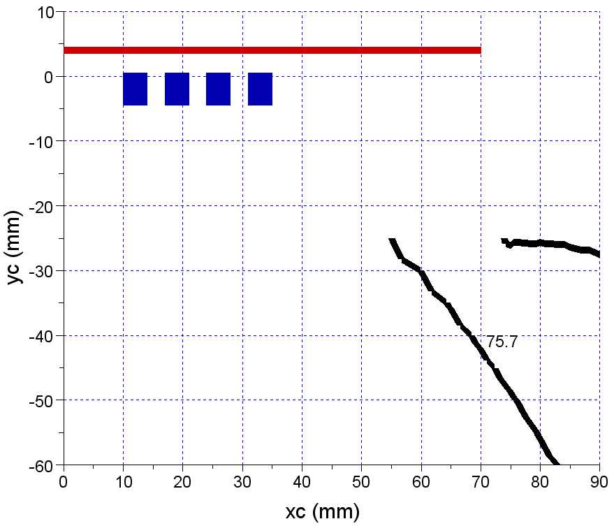 | Figure 16. The voltage phase isoline for aluminium charge |
Figures 17 – 22 shows the positions of the center of sensor coil where the voltage phases on inductor and sensor are the same. The charge materials are steels with permeability 1, 10, 100 and 1000 and with the same resistivity.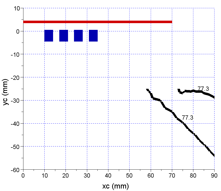 | Figure 17. The voltage phase isoline for a copper charge |
 | Figure 18. The aluminium and copper isolines comparison |
 | Figure 19. Phase dependence on (xc,yc) positions for non-magnetic steel |
 | Figure 20. Phase dependence on (xc,yc) positions for μr=10 magnetic steel as charge material |
In Figure 21, the phase isoline is given for a magnetic steel (μr = 100).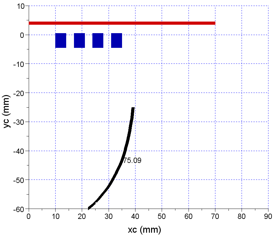 | Figure 21. Phase dependence on (xc,yc) positions for μr=100 magnetic steel as charge material |
Figure 22 contains the phase isoline for the = 1000 magnetic steel as the material of the charge. 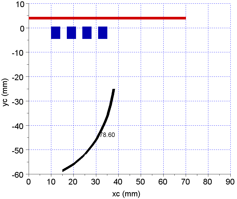 | Figure 22. Phase dependence on (xc,yc) positions for μr=1000 magnetic steel as charge material |
In the case of this second inductor, it appears that the isoline position and shape does not vary too much when the charge material magnetic property increases.In Table 2, the active powers in the Charge region are given for all the second part cases.| Table 2. Comparison between actives powers induced in charge [kW] |
| | No charge | Alu- minium | Copper | Steel | | | | | µr=1 | µr=10 | µr=102 | µr=103 | | 0 | 0.91 | 0.65 | 3.7 | 3.5 | 3.1 | 2.1 |
|
|
Figure 23 shows the geometrical place for positions of the center of the sensor for that the value of voltage phase measured is the same with value of the voltage phase on terminals of the induction heating system.Therefore, even for steel with a nonlinear permeability, are some positions where the sensor can estimate precisely the voltage phase. These results prove that is possible to build a measurement system to measure the active power absorbed by an induction heating system based on the proximate magnetic flux. This sensor coil can accurately estimate the voltage phase on the inductor.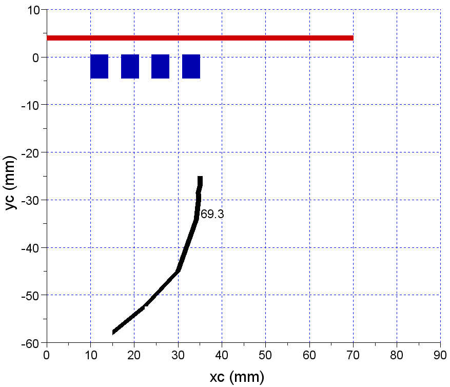 | Figure 23. Phase dependence on (xc,yc) position for magnetic steel with nonlinear permeability as charge material |
5. Conclusions
A method for measuring the active power of an induction heating system in operation in a non – intrusive way was proposed. The finite element models and the simulation results analyzed in this paper prove the existence of positions of coil sensor where the output sensor voltage has the same phase as the inductor supplied voltage. The outcomes are diagrams associated to the induction heating device, containing the voltage phase isolines for different charge materials. As a general rule, the isoline will get closer to the longitudinal inductor if the charge material has a high permeability. The isoline has a value which is much lower than the 90° value. Using these two findings, one can measure the inductor voltage phase by placing the sensor coil as close it can be to the longitudinal inductor coil.
References
| [1] | P. E. Mix, “Introduction to nondestructive testing – a training guide – second edition”, John Wiley & Sons, 2005. |
| [2] | J. G. van Bledel, “Electromagnetic fields – second edition”, John Wiley & Sons, 2007. |
| [3] | B. Thidé, “Electromagnetic field theory – second edition”, Uppsala, Sweden, 2009. |
| [4] | S. Zinn, S.L. Semiatin, « Elements of Induction Heating », ASM International,1988 |
| [5] | U.I.E. “Induction Heating” working group, “Induction heating industrial applications”, 1992. |
| [6] | S. S. Rao, “The finite element method in engineering – fourth edition”, Elsevier, 2005. |
| [7] | E. Pratt , “Power measurements” in “Electronic instrument handbook – third edition”, Clyde F. Coombs, jr. , Mc Graw-Hill, 2000. |
| [8] | Flux 10.3. documentation – The induction heating tutorial |
| [9] | V. Fireteanu, P. Taras, M. Popa, S. Pasca , “Transient Magnetic – Transient Thermal Finite Element Models of Coil and Workpiece Temperature Increase During Magnetoforming Processes” Proceedings of Int. Conference on Electromagnetic Processing of Materials, October 2009 |
| [10] | John G. Webster, The measurement, instrumentation, and sensor – Handbook, 1999 CRC Press. |
| [11] | G. Koranyi, Measurement of power and energy, Technology of Electrical Measurements, 1993, Chichester, John Wiley & Sons |
 Abstract
 Reference
 Full-Text PDF
 Full-Text HTML