-
Paper Information
- Paper Submission
-
Journal Information
- About This Journal
- Editorial Board
- Current Issue
- Archive
- Author Guidelines
- Contact Us
American Journal of Economics
p-ISSN: 2166-4951 e-ISSN: 2166-496X
2023; 13(1): 25-33
doi:10.5923/j.economics.20231301.03
Received: Jan. 9, 2023; Accepted: Jan. 30, 2023; Published: Feb. 25, 2023

Effects of Population Growth on the Availability of Agricultural Products in Burundi
 Abstract
 Reference
 Full-Text PDF
 Full-text HTML
Bizimana Egide1, Ntakirutimana Leonard1, 2, 3, Nimenya Nicodeme1, Gahimbare Mbaye Larissa2
1Faculty of Agronomy and Bioengineering (FABI), University of Burundi (UB), Bujumbura, Burundi
2High Institute of Business (ISCO), University of Burundi, Bujumbura, Burundi
3Bureau of Strategic Studies and Development (BESD), Bujumbura, Burundi
Correspondence to: Ntakirutimana Leonard, Faculty of Agronomy and Bioengineering (FABI), University of Burundi (UB), Bujumbura, Burundi.
| Email: |  |
Copyright © 2023 The Author(s). Published by Scientific & Academic Publishing.
This work is licensed under the Creative Commons Attribution International License (CC BY).
http://creativecommons.org/licenses/by/4.0/

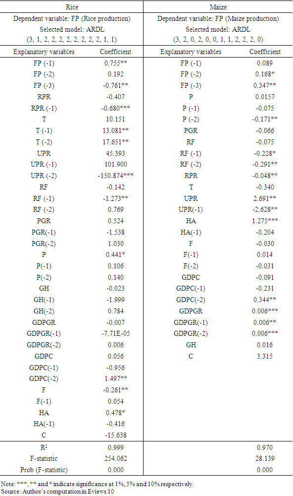
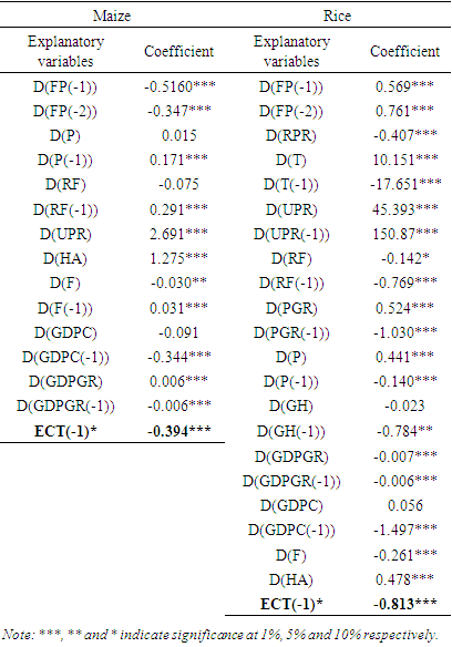
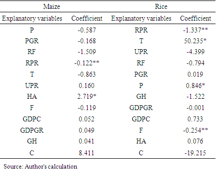
Food availability and population growth have long been of concern to researchers. Using ARDL model and bounds co-integration test for estimating the impact of population growth in both short and long run in Burundi, the findings showed that ECT is negatively significant for both items at 1% level and therefore the long run equilibrium can be reached. Annually, the coefficient of ECT for maize production is equal to -0,394 meanwhile this for rice production is equal to -0,813. Population growth (PGR) is a major factor in food availability because when this variable increases by one unit, in the short term, rice production increases by 0.524%. But the increase of one percent of rural population (RPR) in the first instance implies a decrease of 0.407% of rice in the short term. However, in the long term, increasing this variable by one percent implies a reduction in production of 0.122% for maize and 1.337% for rice annually. For the long run, the contribution of the population growth (PGR) is not significant for the two items and sign is different from one to another.
Keywords: Population growth, Food availability, Lags, ARDL
Cite this paper: Bizimana Egide, Ntakirutimana Leonard, Nimenya Nicodeme, Gahimbare Mbaye Larissa, Effects of Population Growth on the Availability of Agricultural Products in Burundi, American Journal of Economics, Vol. 13 No. 1, 2023, pp. 25-33. doi: 10.5923/j.economics.20231301.03.
Article Outline
1. Introduction
- The availability of sufficient food for a growing population is a major concern in both developed and developing countries. In his Essay -Principle of Population- Malthus (1798) indicates that food scarcity is an important problem for the growing population of the globe. Thus, he developed a theoretical framework between the productive capacity of the earth and population growth. He concludes by saying that the power of population is infinitely greater than the power of the earth to produce the sustenance of man. The environmental reality testifies that the availability of drinking water and arable land is becoming scarce while the population is growing at a constant rate. This alarming increase in population places human beings in a universal famine as Malthus asserts in his Essay; which is also the current case according to FAO et al. (2015) the cause of the increase in the number of undernourished people in the world.Moderate population growth has positive effects on long-term living standards in both developed and developing countries compared to steady or rapid population growth. This seems obvious from the fact that each additional person exerts a pressure of needs on their parents, society and the environment (Simon, 2012). Some authors such as Simon (2014) point out that the empirical data does not support this single a priori view of Malthus using concrete historical examples; population growth can be an asset for developing countries. But the most important phenomenon in the study of population is the change in population size because it affects the resources available to people. The wealth of a group of people or their offspring (in food, manufactured goods, space and other resources) is strongly correlated with the size of the population. Resources are the main reason why the study of population is important, and resources are the subject of economics.On a global scale, the African continent is experiencing galloping population growth and more particularly sub-Saharan Africa. The countries of the EAC bloc come in the closest ranks of countries with strong growth, including Uganda in the first place with its 5th place followed by Burundi (9th place) with a rate of 2.94% in 2020. In This region, experiencing accelerated population growth, is also experiencing a very pronounced rate of undernourishment as in four people one person suffers from undernourishment (Rabin, 2011; Hall et al., 2017).While the population increases with exponential growth, the resources do not keep peace. This effect has multiple repercussions on this same population and on the environment since the increase in population implies an increase in the demand for goods and services, which implies additional pressure on the environment (Guillebaud & Hayes, 2008). As production does not keep pace with the population, an unprecedented increase in different forms of malnutrition is observed in different age groups of the social fabric. Aware of this phenomenon, man seeks to terminate this deficit by intensification and industrialization, which leads to the erosion of biodiversity and the environment in general either by pollution (emission of GHGs and soil pollution) or by extension of arable land (implication on deforestation), etc. (UNDP, 2012). This phenomenon places us right in the face of a snowball effect that the human race will no longer be able to stretch except by becoming aware. This paper shows the (non-exhaustive) effects of population growth in Burundi on the availability of rice and maize.
2. Literature Review
- A vast literature exists on the relationship between food security and population growth. According to Ahmad & Ali (2016) agricultural production depends mainly on natural resources, the performance of the agricultural sector, public investments and incentives for private farmers in the provision of rural health care and R&D plan funded by the private sector (NGOs) and spillovers from intervention products to significantly strengthen the agricultural productivity sector. Where some researchers have given more importance to agricultural inputs to explain agricultural productivity, other economic research has gone so far as to include the contribution of human capital in their analyzes (Antholt, 1994; Beal, 1994; Evenson and McKinsey, 1991; Jamison and Lau, 1982; Nehru and Dhareshwar, 1994; Pardey et al., 1992; Pray and Evenson, 1991; Rosegrant and Evenson, 1992 cited by Zepeda (1995) et Ahmad & Ali (2016)).Sub-Saharan African countries such as Burundi face a series of constraints that increase their vulnerability to the causes and consequences of food insecurity (UNDP, 2012). This region of Africa is well within reach of the SDGs which are the eradication of hunger (“Zero Hunger” in 2030) and the achievement of food security, as is the case for the achievement of food security on a global scale, especially in the era of the Anthropocene and more accelerated population growth. A very simple and striking fact, it is estimated that in 2050 the African population will be multiplied more than twice between 2015 and 2050 (it will increase from 1.1 to 2.4 billion), and even more for some of the poorest countries, including Angola, Burundi, Democratic Republic of Congo (DRC), Malawi, Mali, Niger, Somalia, Uganda, Tanzania and Zambia, a five-fold increase is expected between 2015 and 2100 (UN, 2015), which leads to urbanization and parceling, thus reducing cultivable land such as the constructions observed today in the rice-growing region of the Imbo plain and will continue, which does not exclude effects on production, food demand and directly on food security (Christiansen, 2009). According to Hall et al. (2017) such a dramatic population increase in these countries will make it even more difficult to eradicate poverty, social inequality, hunger and malnutrition.However, faced with this state of affairs of loss of production, man seeks to compensate for this deficit by conquering new, more productive virgin lands such as forests to relaunch the growth of the agricultural sector (Degand & Lefebre, 1980; Tachibana et al., 2001) by extension of arable land, which is the case for African countries (NEPAD, 2013; OCDE, 2016). This deforestation and overexploitation of the soil have the main consequences of pollution and impoverishment (of the soil) as well as climate change. To this, let us add that urbanization supports food availability and increases the share of GDP through the development of the secondary sector, which is synonymous with pollution.
3. Research Methodology
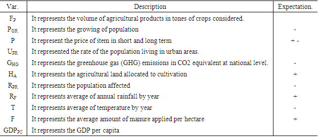
- Definition of variablesThe data we used come from the sites of the FAO, the World Bank (World Bank Indicator) as well as the climate change knowledge portal (CCP). The period of analysis extends from 1966 to 2018. For the case of our paper, we analyzed the effect of population growth (PGR) on the availability of main food products (FP)1 in Burundi such as corn and rice. The choice of these two commodities is not the result of chance. These two cereals are staples of human nutrition in East Africa (Macauley & Ramadjita, 2015). PGR being the variable of interest, we used other determinants of food availability as control variables.
|
 | (1) |
 Where
Where  is a matrix of integrated order
  and
and  dimension variables that are not cointegrated with each other,
  and
and  are series of uncorrelated errors with zero means and constant variance-covariance matrices and
  is the dimension matrix of the coefficients such that the vector
  of the autoregressive process in
  is stable. Or implicitly:
 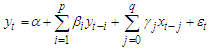 | (2) |
 represents the short run effect of
  on
on  while the long run effect of de
  on
on 
 is obtained by making a computation from the following relationship:
 And then we get:
 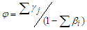 The estimating equation is then given by:
 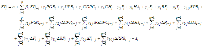 | (3) |
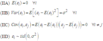 The first hypothesis implies a good distribution of the point cloud of the sample on either side of the regression. The second assumption implies that the error terms are homoscedastic (i.e. the variance remains constant) and the third states that they are non-auto correlated (i.e. the covariance is zero). In the opposite case of the last two hypotheses, the terms are said to be heteroscedastic for IIB while they are said to be auto correlated for IIC. The IID hypothesis translates that the error terms have a normal distribution with zero mean and constant variance
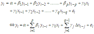
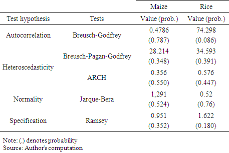
  . In order to validate our model, we performed tests on the residuals of the estimated model. These include tests for normality (Jarque-Bera statistic), autocorrelation (Breusch-Godfrey), heteroscedasticity (Breusch-Pagan- Godfrey and the ARCH test) and specification (Ramsey).Bounds cointegration testThis test aims to examine the existence or not of a long run relationship between the variables. The approval of the cointegration hypothesis implies the existence of a long run equilibrium relationship between the variables. The classic cointegration tests as presented by Engle & Granger (1987) and Johansen (1988) are not up to serving for our case since they assume that the variables are integrated of the same order. This is how Pesaran et al. (2001) presented a test that is suitable for mixing the embedded variables of different order I(0) and I(1). It is a test based on the Fisher test which, in its null hypothesis, assumes the joint equality of the coefficients. The cointegration test at the bounds (I(0) and I(1)) is performed in order to establish a long run relationship between the variables. Each sample variable is taken as a dependent variable in the calculation of this test (Narayan, 2005; Nkoro & Uko, 2016). The cointegration testing approach of our ARDL model is given by the following equation:
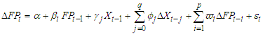 | (4) |
 is the difference operator,
  and
and  are the coefficients of long run while
  and
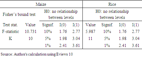
and  are the parameters of short run. This specification presents the ARDL model as either an error correction model (ECM) or a vector error correction model (VECM). This then assumes the existence of cointegrating relationships between the variables. Indeed, the test is done in two stages, namely:- Determine the optimal shift first and foremost using an information criterion of choice;- Use Fisher's test to test the hypotheses:
 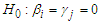 .- The test procedure is that one must compare the Fisher values calculated with the critical values (limits) tabulated at the different thresholds by Pesaran et al. (2001).It should be specified that the lower limit takes the critical values of the variables integrated in level I(0) while the upper limit takes the values of the variables integrated in first difference I (1). Thereby:- If the calculated Fisher statistic > upper bound: existence of cointegration;- If the calculated Fisher statistic < lower bound: cointegration does not exist;- If upper bound < calculated Fisher statistic < lower bound: no conclusion.Short run and long run relationship The concept of cointegration between variables leads to a representation of an ARDL model in the form of an ECM or a VECM. The ECM is a representation of the dynamics of a linear time series in terms of its level and a shift polynomial in the differences. Its coefficient represents the restoring force or speed of adjustment to long-term equilibrium. Following (Pesaran, 2016) and starting from our model equation, the ECM can be represented as follows:
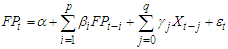 | (5) |
 representing the matrix of all the explanatory variables of the model, we then have this equation which can be rewritten as follows:
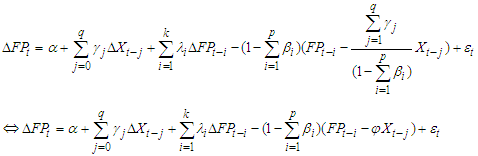 | (6) |
 at the moment
  is the coefficient of the slope of the relationship of long run
  on agricultural production
  . The preceding relation is known as the error correction representation of the ARDL (p, q) model. The term
  is called derivative effect while
 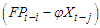 is error correction term (ECT). Its coefficient shows how much the imbalance is corrected, that is, the extent to which any imbalance from the previous period is adjusted in the dependent variable. A positive coefficient indicates divergence, while a negative and significant coefficient indicates convergence.
4. Results Presentation
- Stationarity of model variablesIn time series analyses, several problems have been identified including the problem of "stationarity" which results in spurious regressions (Granger & Newbold, 1974) if not given more attention. To do this, Dickey & Fuller, (1979; 1981) recommended performing stationarity tests before any study on time series. Thus, the following table shows the level of stationarity of each variable of the model.
|
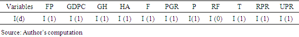
|
5. Results of Diagnostic Tests of Estimated Models
- The estimated models are statistically significant and the explanatory variables taken into the models contribute more than 90% in determining the production of the two crops considered. The residuals of the models are then tested and the results show that no test is significant at the 5% level. The following table shows the results of the diagnostic tests of our models estimated above.
|
|
|
|
6. Conclusions and Recommendations
- In Burundi, the growth of production generated by population growth is not effective knowing that high population growth is observed in rural areas while this large part of the population negatively affects agricultural production due to of the highest dependency ratio but also it decreases the share of production per inhabitant which is the source of capital as well as a good proxy for food accessibility. The fragmentation of land caused by higher population growth leads to excessive exploitation and the use of more mineral fertilizers depleting the soil more and more in the long term, which causes a drop in production. The higher population growth is therefore not good news for the maintenance of food security, rather the urbanization accompanied by the development of the secondary sector even if it is still at an embryonic stage in Burundi.The government should therefore put in place a new land use planning policy by creating villages in order to remedy the problem of land fragmentation and a birth control policy in order to end the food deficit. It should also make a price stabilization policy, guarantee a remunerative producer price; especially for corn. Since overall economic growth is not positively correlated with the growth of agricultural production, we should see how to increase the budget allocated to the agricultural sector and increase initiatives in Research and Development oriented in the agricultural sector.With regard to the mainly rural population, change mentalities on the old sayings around the child (the child is a wealth "Umwana ni itunga" or the child is a blessing "Umwana ni umugisha") which illustrate that a high number of children brings more happiness while ignoring that they are also a burden for them as well as for society in general. Producers should also feel the need to use organic or organo-mineral manure to boost production and restore the fertility of poor soils.For the scientific community, I recommend that such a study be conducted using short frequency data as soon as it becomes available and also expand the study area to confirm the authenticity of the results of this study.
Note
- 1. Data is logarithmically transformed.