Taibi Boumedyen1, Lamri Khadidja2
1MECAS Laboratory, Department of Economics, University of Saïda, Algeria
2ITMAM Laboratory, Department of Economics, University of Saïda, Algeria
Correspondence to: Taibi Boumedyen, MECAS Laboratory, Department of Economics, University of Saïda, Algeria.
| Email: |  |
Copyright © 2021 The Author(s). Published by Scientific & Academic Publishing.
This work is licensed under the Creative Commons Attribution International License (CC BY).
http://creativecommons.org/licenses/by/4.0/

Abstract
This study aims to analyze the relationship between the tourism sector and economic growth in some Mediterranean countries using Panel data for 25 observations, as the most important characteristic of this study is taking into account the dynamic character of the tourism sector and economic growth, given that it matches the development defined by econometric modeling using time-series data for longitudinal data. The results of the study concluded that there is a long-term relationship between the number of tourists, the exchange rate and economic growth in the countries of the study sample.
Keywords:
Tourism, Economic growth, Panel data
Cite this paper: Taibi Boumedyen, Lamri Khadidja, Panel Data Analyses of Tourism Industry and Economic Growth in Some Mediterranean Countries from 1995-2019, American Journal of Economics, Vol. 11 No. 2, 2021, pp. 64-70. doi: 10.5923/j.economics.20211102.03.
1. Introduction
Tourism has achieved high growth rates in recent years, and this will increase the gross domestic product for each country, representing about 10.4% during 2019, as tourism is considered a source of attraction of foreign currencies in the national economy and is considered the largest attraction for investments, especially investment in the rehabilitation of the natural environment and cultural implications.Tourism is one of the most important sectors affected by the Corona pandemic, which led to its deterioration, especially since this sector has a close relationship with operating levels and official reserves and foreign exchange proceeds, and in this regard many travel agencies around the world have canceled flights, which negatively affected its revenues.Tourism is one of the most important economic activities in the Mediterranean countries "some countries from Europe, Asia and Africa "The mild climate, stunning scenery and rich historical heritage make the Mediterranean an ideal holiday destination for millions of tourists from all over the world.In this sense, our problem is:What is the impact of the tourism sector on economic growth in some Mediterranean countries?We proposed two main hypotheses for our research, which are:1. The increase in the number of tourists has a positive effect on economic growth in some Mediterranean countries.2. The devaluation or depreciation of the Algerian currencies has a positive effect on the economic growth in some Mediterranean countries.Among the previous studies dealing with the relationship between the tourism sector and economic growth / Nikolawos Dritsakis (2012), Can Tansel Tugcu (2014) Govdeli Tuncer & Baskonus Direkci Tuba (2017), Gueye Thierno Ndao & others (2020).- Nikolawos Dritsakis (2012): This study aims to analyze the relationship between economic growth and tourism development in seven Mediterranean countries. Using real tourism per capita, the number of international tourist arrivals per capita, the real effective exchange rate, and the per capita real GDP as variables for the study taking into account the annual data for the period 1980-2007. The tests of panel cointegration and fully modified ordinary least squares (FMOLS) are conducted, using panel data. (Dritsakis, 2012).- Can Tansel Tugcu (2014): This study aims to analyze the relationship between tourism and economic growth in some Mediterranean countries, and investigates the causal relationship between tourism and economic growth in European, Asian and African countries bordering the Mediterranean Sea. This study used the Panel data for the period from 1998 to 2011, and the Granger causality analysis developed by Dumitrescu and Hurlin (2012). The results indicate that the causal trend between tourism and economic growth depends on the country group and the tourism index. Moreover, European countries are better able to grow from tourism in the Mediterranean region (Tugcu, 2014).- Govdeli Tuncer & Baskonus Direkci Tuba (2017): This study aimed to analyze the long-term relationship between tourism receipts and economic growth for the period 1997 - 2012 of 34 OECD countries, using the Panel data, so that the Pedroni and Kao tests for the cointegration were used. The results of this study concluded that increasing tourism revenues had a positive effect on economic growth in the long term in some OECD countries (Govdeli & Baskonus Direkci, 2017).- Gueye Thierno Ndao & others (2020): This study aimed to analyze the relationship between Senegalese tourism constitutes and economic growth. To this end, in a framework of cointegration, two regression models are deployed successively. Therefore, the results of this study concluded that tourism positively impacts long-term economic growth. A 1% increase in tourism receipts would translate into a 0.71% increase in GDP per capita and Granger causality tests proved a one-way trend between these two variables. Senegalese tourism is a driving force for economic growth. Finally, the results also revealed the existence of a positive relationship between the growth of Senegalese tourism and the development of economic sectors such as agriculture and industry (Gueye & others, 2020).
2. Method and Tools
We will try to highlight the most important axes related to the econometric methodology used in the analysis, which include models or data series cross-sectional (Panel data) used in its estimation, when the effects and individual characteristics converge between the study group, as can be found in the models of macroeconomic and study the relationship between macroeconomic variables.Panel data define cross-sectional observations, such as (countries, states, companies, households ...) observed over a given period, “combining cross-sectional data with time simultaneously” (Dielman, 1989, p. 02).In our study of the impact of the tourism sector on economic growth in some countries Mediterranean countries, we chose nine countries as a sample for the study, namely: Algeria, Morocco, Tunisia, Egypt, France, Germany, Spain, Italy, Malta, Israel, and our selection of these countries was related to With the availability of data on the study variables, taken from the database approved by the World Bank, and the study period was chosen from 1995 to 2019.In our attempt to study the impact of the tourism sector on economic growth, the study model is determined as follows: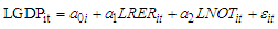 -
-  : The logarithm of GDP for country i in period t, and represents the dependent variable in the model.-
  : The logarithm of the real exchange rate of country i in period t.-
  : The logarithm of the number of tourists for country i in period t.
3. Modeling the Relationship (Tourism Sector, Economic Growth) in Some Mediterranean Countries for the Period 1995-2019
In this section, we will present the econometric results related to the long-term relationship between the tourism sector and economic growth in nine Mediterranean countries.
3.1. Determining the Type of Appropriate Model for the Study Sample Data
In the econometric base we will present the estimated model then, the test of the possibility of a single trace in the model and the test of determining the quality of the effect.
3.1.1. Estimating Study Model
On the basis that the study data are longitudinal, we distinguish three models: 1. Pooled Regression Model (PRM) This model is written as: (Park, 2011).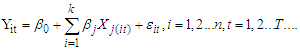 | (1) |
Where: 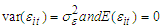 2. Fixed Effects Model (FEM) This model is written as: (Biørn, 2017).
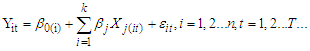 | (2) |
Where:  The fixed-effects model is called Dummy Variables Model Least Squares, after adding the dummy variables D in equation (2) the model becomes as follows:
 | (3) |
3. Random Effects Model (REM) This model is written as: (Pesaran, 2015)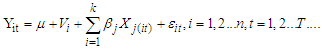 | (4) |
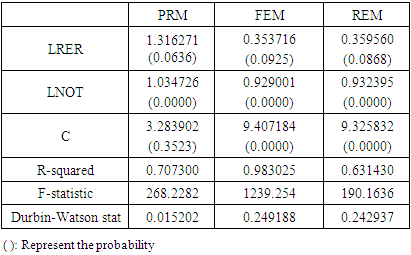
The first and second models are estimated by the least-squares method. The last model is estimated using the generalized least squares method, and the results are recorded in the following table:Table 1. Estimating the PRM, FEM, REM models
 |
| |
|
Through Table 1, we note that the calculated Fisher is greater than the tabular Fisher  , therefore we reject the null hypothesis (the existence of a single effect between countries).
3.1.2. Test for the Possibility of a Single Trace in the Model
First, we test the spatial presence of an individual effect within the data of the study sample, and this is based on a Fisher-type test in which the null hypothesis fits the overall homogeneity model (H0: the absence of any trace of individuals in the studied sample), and the statistic of this test is: (Greene, 2005, p. 277).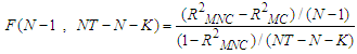 - N: The number of individuals (in our case 09 countries).- T: The length of the proposed time series for the study (in our case, 25 years).-
  : The number of external variables in the model (in our case 2).-
  : Represents the R-squared coefficient of the restricted model, in this case, it is a model without any effect
  .-
.-  : Represents the R-squared coefficient of the restricted model, in this case, it is a model without any effect
  .
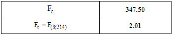
.Table 2. Test for the possibility of a single trace in the model
 |
| |
|
Through Table 2, we note that the calculated Fisher value is greater than Fisher’s statistical value, (347.50 > 2.01) and therefore we reject the null hypothesis at 5% significance, that is, there is an individual effect within the study sample data.
3.1.3. Test to Determine the Quality of the Effect
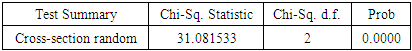
After performing the Fischer test, which showed the presence of the individual effect, we will determine the quality of the effect, using the Hausman Test to choose between a fixed effect model or a random effect, and the result of this test is presented in the following table:Table 3. Hausman Test
 |
| |
|
Through Table 3 we notice that the calculated statistic for Haussmann’s test is large compared to the tabulated statistic 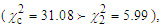 and therefore there is a correlation between the interpreted variables and the individual effect (rejecting the null hypothesis), and therefore the appropriate model for the study sample data is of the type of individual effect and this means that the sample countries agree from the parameters of the variables interpreted and differ in the values of the constant.Thus, the chosen model is:
 Through the above equation, we note that the exchange rate has a positive effect on the GDP, as an increase in the exchange rate by 1% leads to an increase in the GDP by 0.35%, we also found a positive relationship between the number of tourists and the GDP, as an increase in the size of the tourism sector by 1% leads to an increase in the GDP by 0.92%.Through the above equation, a statistical analysis of the results can be presented as follows:- Through the results of the Student test, the estimator’s parameters of the model are significant at a significance level of 5%.- Through the results of the Fisher test, the model is significant at a level of 5%.- The value of the R-squared coefficient has reached and it is an excellent value.- The results of the Durbin-Watson test indicate the presence of a positive self-correlation for errors of the first degree, which makes the estimators of the non-convergents parameters, and this means that the model is not acceptable to the standard.-
  : This is an indication of a false regression in the model, mainly due to the instability of the series.
3.2. Estimate the Long-Term Relationship between the Tourism Sector and economic Growth
In this section, we will present the results of the estimation of the long-term relationship between the tourism sector and economic growth.
3.2.1. Graphical Presentation of Variables
Before any analysis of time series, it is essential to carefully study the graph representing its evolution, because the latter provides a priori a global idea on the nature and characteristics of the processes generating this series, namely the trend, etc.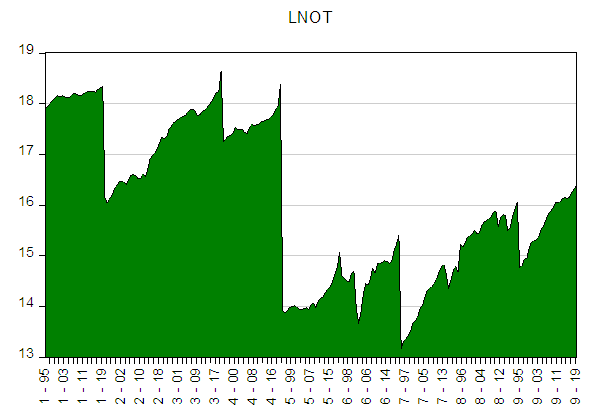 | Figure 1. LNOT |
The graphical representation shows that there is a trend. So probably these series are not stationary, for the confirmation we will apply the stationarity test.
3.2.2. Autocorrelation Test
We notice from the correlation function of the time series (LNOT, LRER, LGDP) that the coefficients calculated for the deviations K=1.2..3… .12, it is outside the confidence domain  , which means that it differs considerably from zero.
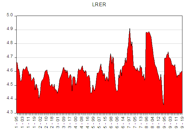 | Figure 2. LRER |
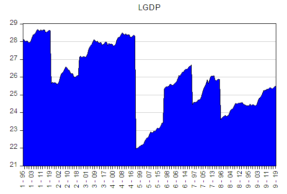 | Figure 3. LGDP |
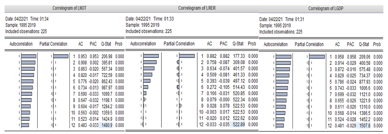 | Figure 4. Autocorrelation test for time series (LNOT, LRER, LGDP) |
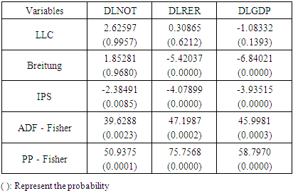
By testing the coefficients of the autocorrelation function for the time series, we found that all the variables have autocorrelation function coefficients that differ significantly from zero, which gives us a first idea of the instability of the time series. To test the stationarity of time series, the following statistical tests were used: Levin, Lin and Chu test, Breitung test, Im, Pesaran et Shin test, and Maddala et Wu test, and the results were shown in the following table:Table 4 Stationarity test of longitudinal time series
 |
| |
|
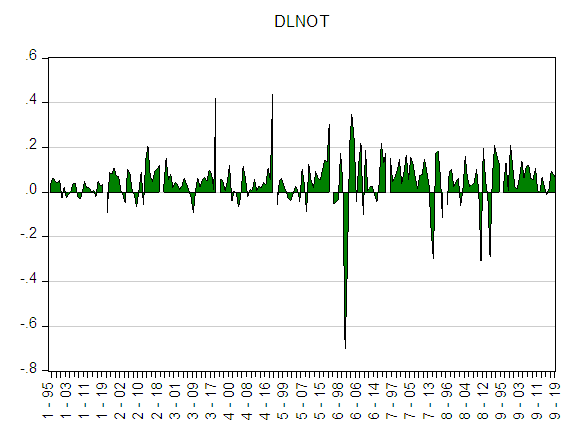 | Figure 5. DLNOT |
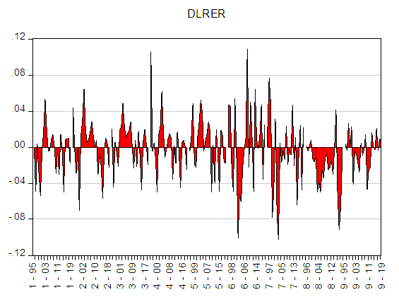 | Figure 6. DLRER |
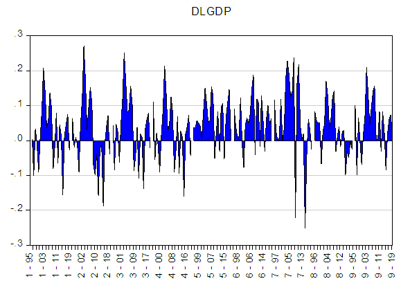 | Figure 7. DLGDP |
According to Table 4, the variables are stationary at the first difference, using at least three statistical tests at the significance level of 5% (See Appendix 01: Time-series are not stationary at the level at the significance level of 5%).Thus, the following figures show the stationarity of the time series at the first difference, and a test of the stationary series at the first difference to ensure stationarity at the level.
3.2.3. Long-Term Relationship to Longitudinal Data
If the variables of the longitudinal data are stable of the same degree, a cointegration test can be performed (Hurlin & Mignon, 2006, pp. 23-28). Among the most important tests in this field are the Pedroni test and the Kao test, and each of these tests is based on the following two hypotheses: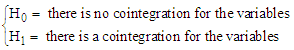
3.2.3.1. Pedroni Test
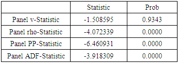
Pedroni test results are shown in the following Table: Table 5. Pedroni test
 |
| |
|
Through Table 5, we notice that the majority of the Pedroni test statistics have proven that there is cointegration between the variables 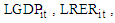
 at the level of significance of 5%. Based on this result, we can estimate the long-term relationship, and then the estimated relationship between the variables represents a long-term structural equilibrium relationship and not a false regression.
3.2.3.2. Kao Test
Kao test results are shown in the following Table: Table 6. Kao test
 |
| |
|
Through Table 6, we note that the results of the Kao test proved that there is cointegration between the variables at the level of significance of 5%, and thus the long-term relationship can be estimated, and the estimated relationship between the series of cointegration becomes like a structural equilibrium relationship in the long run and not a false regression.The estimated model is called the vector error correction model (VECM).
4. Estimation of Error Correction Model with the FMOLS Method
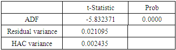
To estimate the VECM for long-term relationship we use the FMOLS method developed by Pedroni (2000).Table 7. Estimation of Error Correction Model with the FMOLS method
 |
| |
|
Through Table 7 we found that the estimator’s parameters the  is statistically acceptable at the significance level of 5% and its sign is economically acceptable and has an impact on determining the GDP in the long term, as an increase in the size of the tourism sector by 1% leads to an increase in the economic growth rate by 1.00% Thus, it can be considered as one of the determining factors of the GDP, and we explain that the number of tourists has an impact in the long term.As for the estimator the
  it has little influence in determining the GDP in the long term, due to the inability of the exchange rate to form the GDP for the countries of the study sample.It also shows the value of the R-squared
  , that is 98% of the volatility in GDP is explained within this model in the long term.
5. Conclusions
The study aimed to measure the impact of the tourism sector on economic growth in some Mediterranean countries during the period 1995-2019 so that the Panel data was used through the application of 3 models: the pooled regression model(PRM), and the fixed effects model(FEM) and Random Effects Model (REM).The results of the study of the impact of the tourism sector on economic growth in some Mediterranean countries reached the following:- The proposed model for the study is the fixed effect model, through the statistical (R-squared, Fisher test) and economic (the significance of the coefficients) evaluation of the Haussmann test.- By determining the type of individual effect, it became clear that it is fixed, meaning that it is determined based on of each country, this is economically acceptable, but this model was rejected due to the existence of the autocorrelation of errors (DW = 0.01).- The results showed that the longitudinal time series are stationary and integrated with the first degree, therefore the search for the existence of a cointegration relationship in the long run was done using the Pedroni and Kao tests. Thus, the tests confirmed the existence of a cointegration relationship in each of the countries of the study sample.- The NOT, the RER, and the GDP have a positive effect on economic growth in the long run.- Using the FMOLS method, the validity of the relationship was accepted, based on the results of the assessment, an increase in the value of the currency exchange rate by 1% leads to an increase in growth by 0.31%, as well as an increase in the tourism sector by 1% leads to an increase in growth by 1.00%.- Finally, the results showed that 98% of the volatility in GDP is explained within this model in the long term.
Appendix
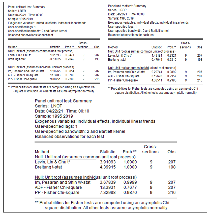 | Appendix 1. Stationarity test of time series at the level |
References
| [1] | Biørn, E. (2017). Econometrics of Panel data methods and applications. United Kingdom: Oxford. |
| [2] | Dielman. (1989). Pooled Cross-Sectional and Time Series Data Analysis. USA: Texas Christian University. |
| [3] | Dritsakis, N. (2012). Tourism development and economic growth in seven Mediterranean countries: a panel data approach. Tourism Economics. |
| [4] | Govdeli, T., & Baskonus Direkci, T. (2017). The relationship between tourism and economic growth: OECD countries. International Journal of Academic Research in Economics and Management Sciences. |
| [5] | Greene, W. (2005). économétrie. Paris: Université Paris II. |
| [6] | Gueye, T. N., & others. (2020). Tourism and inclusive economic growth in Senegal. Benchmarks and Economic outlook. |
| [7] | Hurlin, C., & Mignon, V. (2006). , une synthèse des testes de cointegration sur données de Panel,. Université d’Orléans. |
| [8] | Park, H. M. (2011). Practical guides to panel data modeling: A step by step analysis using stata. Japan: Management & Policy Analysis Program. |
| [9] | Pesaran, H. (2015). Time Series and Panel data Econometrics. United Kingdom: Oxford. |
| [10] | Tugcu, C. T. (2014). Tourism and economic growth nexus revisited: A panel causality analysis for the case of the Mediterranean Region. Tourism Management. |

 Abstract
 Reference
 Full-Text PDF
 Full-text HTML