Brian Kapotwe1, Gelson Tembo2
1Directorate of Research and Graduate Studies, University of Zambia, Lusaka, Zambia
2Department of Agricultural Economics, University of Zambia, Lusaka, Zambia
Correspondence to: Brian Kapotwe, Directorate of Research and Graduate Studies, University of Zambia, Lusaka, Zambia.
| Email: |  |
Copyright © 2021 The Author(s). Published by Scientific & Academic Publishing.
This work is licensed under the Creative Commons Attribution International License (CC BY).
http://creativecommons.org/licenses/by/4.0/

Abstract
The ensuing assessment is on whether Zambia's persistent Least Developed Country (LDC) status has a bearing on its vulnerability to the Middle Income Trap (MIT). Using an adapted unit root model, Granger causality tests were conducted to establish which variables affect Zambia's GDP per capita income level and predispose it to the MIT. Thus, per capita income, labour productivity, agriculture share to GDP, and manufacturing industry share to GDP were investigated. The results have shown that agriculture share of GDP strongly affects GDP per capita income while manufacturing share of GDP has a weaker effect on GDP per capita. The results further indicate that changes in agriculture share of GDP strongly affects the manufacturing output. Therefore, Zambia should increase investment in agriculture and manufacturing to maintain a positive GDP per capita income growth and to catalyze growth in the secondary sectors.
Keywords:
Middle Income Trap, GDP, Per Capita Income, Sub-Saharan Africa
Cite this paper: Brian Kapotwe, Gelson Tembo, An Analysis of the Factors Affecting Zambia's GDP Per Capita, American Journal of Economics, Vol. 11 No. 1, 2021, pp. 19-30. doi: 10.5923/j.economics.20211101.03.
1. Introduction
At independence in 1964, Zambia started as a prosperous country but subsequently declined to a low-income country for a long time before graduating to low-middle-income status. To achieve high-income status, a country has to undergo various economic development stages. There are three stages of economic growth in literature: structural transition, the transformation of the economy, and urbanization. Rostow (1960) proposed a five-stage economic development process, including traditional society, transitional stage, take off, and drive to maturity and high mass consumption. By reviewing the country's growth trends and context, this article aims to identify the factors that may predispose Zambia to the Middle Income Trap (MIT). GDP per capita is an essential factor when ascertaining a country's economic growth in relation to its population. The World Bank uses GDP per capita income thresholds to classify countries in three income levels: Low, Middle and High-Income Countries. Understanding the factors that may affect a country's GDP per capita income level could provide a pathway to escaping the MIT. Although there is no universal definition of the MIT, it is generally agreed that countries tend to experience slow growth when they reach middle-income level as they transition from resource-driven growth to growth based on economic efficiency.To the contrary, the convergence hypothesis predicts that Least Developed Countries (LDCs) per capita income would grow faster than developed nations due to higher returns on capital and benefits from using imported technology and skills. While the economic theory does not provide precise predictions about the convergence or divergence path, it does detail a set of factors that could determine whether a specific country will take a convergence or divergence path.A critical condition for convergence is the existence of decreasing returns to scale in capital markets. According to Fuente (2002), output grows less than proportionally with the capital stock. As a result, this factor's marginal productivity decreases with its accumulation and reduces both willingness to save and the overall economic growth. The second factor to consider about the convergence or divergence of Income per capita or productivity is technological progress. Thus, countries' long-term growth rate will not be the same if they differ in their intensity to develop or adopt new technologies. The following section provides a detailed theoretical and conceptual analysis of growth theories and the MIT. The conceptual framework presents a foundation on the determinants of GDP per capita. Theoretical and conceptual frameworkMany studies use GDP per capita when analyzing economic growth. GDP per capita is the major variable used to determine whether a country is in the Middle-Income Trap (MIT). Eichengreen (2011) and Eichengreen et al. (2013), defined the MIT in absolute terms. According to them, a country experiences a growth slowdown when: (1) the average annual GDP per capita growth rate is 3.5% or above; (2) when growth rate is lower by 2 percent; and (3) when per capita income is greater than $10,000.Economic growth theoryThe changes in the GDP per capita growth rate of countries are explained by economic growth models mainly based on the neoclassical exogenous model by Robert Solow (1956). According to the model, GDP per capita growth rate is higher when countries first accumulate capital. A fundamental assumption in the Solow model is the diminishing marginal product to capital. According to the model, the more capital is accumulated, the less additional output is produced. Thus, developing countries' per capita income is expected to grow faster than developed countries, leading to per capita income convergence. The model highlights that income convergence is due to better chances for growth available to developing countries such as technology from developed countries and higher capital returns.However, growth theory also stresses that there is a limit to the increase in GDP per capita depending on technology level. Only advancements in technology can lead to a positive increase in GDP per capita. Improvements in technology indicate that a country's production mode is moving towards knowledge-intensive, which will result in further improvement in GDP per capita. Therefore, low GDP per capita in less developed countries is due to two main factors. Firstly, the economy is mainly driven by labour-intensive production modes, secondly, due to underdeveloped technology. Therefore, developing countries can improve per capita output by adopting capital or knowledge-intensive production modes. A country's ability to adopt capital and knowledge-based production depends on its stage of development. The structural transformation theory explains the structural changes of an economy and how a given country can maximize growth. The structural transformation of the economyStructural change models are systems by which underdeveloped nations transform their local economy from a heavy emphasis on traditional sectors, i.e. agriculture to more industrial and service-led growth. As a country's economy grows, the agriculture share of GDP is surpassed by the secondary sectors. The model implies that the agriculture sector's growth is key to the overall development of the country. The Lewis two-sector surplus model is an example of the structural-change approach. The model postulates that the agriculture sector fuels rapid industrial growth by utilizing its cheap produce and labour. In this approach, Lewis emphasized the role of agriculture as a labour source for other industries. Justin Lin et al (2018) analyzed the interactions between production led growth and service-led growth. They point out that that production led growth is mainly fuelled by the agriculture sector in developing countries. The study concluded that production led growth is asymmetric at different levels of a country economic development. Justin Lin et al (2018), recommended that to escape the MIT, government intervention is required to prevent premature de-industrialization and sustain the early development process. Economic development requires the re-allocation of production factors from low productivity growth in the primary sectors to a more commercial industrial driven development based on high productivity and returns. According to Lewis, labour and savings have to be retrieved from agriculture to meet capital investments required by the industrial sector. This is why agricultural and industrial development always move hand in hand. While agriculture is important in the intial development stages of a country, recent studies have highlighted the several challenges limiting the full exploitation of agriculture by developing countries. According to Namalguebzanga C.K (2016), although agriculture produce can be used to develop manufacturing in Africa, several obstacles exist. Many African countries have limited practical and vocational skills, low exchange rate management, inadequate infrastructures, and technologies to stimulate agriculture development. The Lewis Model of DevelopmentAccording to the Lewis model of economic development, a country's economy consists of two sectors, namely; agricultural and rural subsistence and industrial, urban, and capitalist sectors. The subsistence sector has a large population relative to products such that the marginal productivity of labour is low to zero. As such, there is 'disguised unemployment'. This can also be a potential reservoir of labour supply to the capitalist sector. When labour supply exceeds demand, the labour market becomes favourable for capitalists who can keep the wage constant. The Lewis model assumes that labour is unlimited that the capitalists will have a constant supply of labour at the same wage. The utilization of excess labour occurs through urbanization as farm workers move to cities in search of work. The incorporation of surplus labour is one way of transforming a country's production mode from labour-intensive to capital intensive. For the capitalist sector, labour is utilized to where the marginal product is equal to the wage not to reduce the capitalist surplus. As a result labour supply exceeds demand and the wage remains constant, leading to profit maximization. Gang Gong (2016) refers to the two stages as 1), digesting surplus labour and 2) the catching-up technology process. He argues that a country would grow rapidly to attain middle-income status during the digesting surplus-labour stage and transform its production from labour-intensive to capital-intensive. The inability to successfully transition from labour intensive to capital intensive mode of production is the reason for the MIT. According to Gang Gong (2016), a country can only escape the MIT if the production mode successfully transforms from capital-intensive to knowledge-intensive. Economic growth theory and the Middle-Income TrapIn view of the above discussion, it is clear that a developing country undergoes two main economic development stages. The MIT is caused by a failure to transition from the first economic stage to the second. When surplus labour is exhausted in the second stage, technological progress or increase in total factor productivity is the only factor that can drive economic growth. Thus, the rate of economic growth would decrease as the economy enters the second stage. Further, technological advancement is also transformed and the improvements in total factor productivity are slower in the second stage. During the second stage, a country is expected to innovate and develop new technologies and not merely import it. The development level difference means that a developing economy can simply import and imitate technologies from developed economies in the first stage were technological progress does not depend on local research efforts. During this stage, technological progress depends on a country's ability to innovate, the reason why technological progress is complex in middle-income countries. This is the main reason for the MIT. The MIT can also be caused by a country's inability to benefit from the subsistence sector and excessive labour utilization. In this case, an investigation into the factors affecting GDP per capita in relation to a country's development level would help define ways of avoiding growth slow down and the MIT. As highlighted in the structural change model, most developing countries in sub-Saharan Africa are still in the transitional stage were agriculture is key to their economic development. Excess labour and savings have to be retrieved from the agriculture sector in order to fuel industrial development. Several authors have found strong evidence indicating that Agriculture is a vital engine for economic growth in developing countries: Titus O. Awokuse, (2008), Joseph Phiri, et al. (2020). In line with the stages of growth theory, agriculture plays a vital role in developing countries' initial development process. It is the primary source of income for the rural population and a precondition for the growth of the secondary sectors such as industry and services. Cenap Ilter (2017) identified four variables affecting GDP per capita in 40 countries: population, GDP, transparency, and compulsory education. Other studies indicate that agriculture and manufacturing have a strong influence on GDP per capita growth rates (Manak Singariya et al. (2015). Manak argues that the shocks from the agriculture sector spill over to GDP per capita and manufacturing. According to Dan Su and Yang Yao (2018), a decline in the manufacturing sector negatively affects an economy's service sector. They note that manufacturing provides an incentive for savings and can also accelerate the rate of technological progress. Qunhui Huang et al. (2017) investigated the experience of high-income Asian economies focusing on the size and productivity of manufacturing, during when they were in and out of the middle-income level. They found that (1) manufacturing share of GDP of the selected economies, keeps on increasing as per capita income grows, (2) despite the relative size, the drastic improvement in the productivity of manufacturing by industrial restructuring is prominent. Jack Jones Zulu, et al. (2018) found that labour productivity impacts South Africa and Mauritius's economic performance. In this study, they argue that investments in physical capital have a positive impact on labour productivity. Determinants of GDP Per capita IncomeFrom its computation, GDP per capita is primarily influenced by population and GDP. Therefore, GDP per capita indicates how a country's economy is growing with its population. PopulationWhen population is analyzed, the GDP per capita measure indicates a country's productivity level per person. As such, variables such as level of education, employment and health status are important. Several studies have been done to assess the impact of population changes and the MIT. Ha and Lee (2016) provide a framework for the analysis of a demography-driven middle-income trap. They focus on the key variable that effectively summarizes demographic structure: the support ratio or effective workers' ratio to effective consumers.Ha and Lee (2016) argue that, in the early stages of development, Asia's fast demographic transition raised support ratios that created a huge demographic dividend, thereby encouraging Asia's fast convergence and economic development. However, in later stages, low fertility, which economic development brought about through the quantity-quality trade-off, eventually leads to falling support ratios and negative demographic dividend. If the support ratio falls to a level too low to catch up with the frontier, the economy can get into a non-convergence trap.Gross Domestic ProductGDP as a measure of a country's economic output is dependent on several variables. GDP comprises all purchases of goods and services produced by a country and services used by individuals, firms, foreigners and the governing bodies. As highlighted above, economic growth in a low-income country is mainly from primary sectors such as agriculture and tends to shift to secondary sectors as the economy transitions to middle-income status. This is because growth can no longer be sustained by the exploitation of physical and human capital resources. Growth should be driven by increased productivity through better technology, innovation and technical skills. Based on this background, the GDP per capita of a newly classified middle-income country is highly dependent on the primary and secondary sectors as well as variables that may affect the population such as education and health.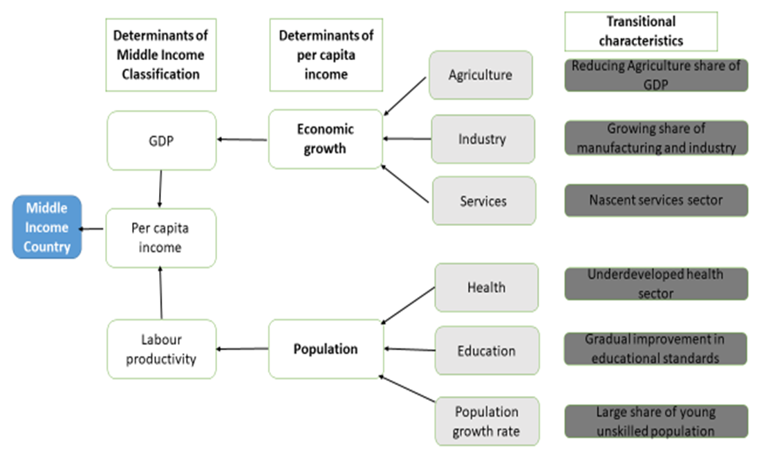 | Figure 1. Determinants of GDP and GDP per capita (Source: Author) |
As highlighted in Figure 1, assessing the variables influencing a country's GDP and GDP per capita would indicate whether the country is likely to get stuck or not. As per Figure 1, four variables were assessed, including agriculture and manufacturing share of GDP, the manufacturing share of GDP, labour productivity, and GDP. These variables are specifically crucial for Sub-Saharan African countries that largely depend on agriculture and natural resource endowments.According to the NEPAD report on agriculture in Africa (2013), agriculture accounts for a considerable portion African's GDP countries and contribute towards major continental priorities, such as eradicating poverty and hunger, boosting Intra-Africa trade and investments, rapid industrialization and economic diversification, sustainable resource and environmental management, and creating jobs, human security and shared prosperity.In addition, most African economies have underdeveloped support systems necessary to develop a productive workforce and avoid the middle-income trap. The educational provisions within any given country represent one of the main determinants of the composition and growth of that country's output and exports and constitute an essential ingredient in a system's capacity to borrow foreign technology effectively. Overview of Zambia's economic performance (1960-2019)To establish the country's economic development stage, the study reviewed Zambia's economic performance for the period 1960-2019. Understanding the stage of economic development is key to assessing the country's vulnerability to MIT. While Rostow (1960), proposes five stages of economic development, many development economists still maintain that there are three main stages including a) a structural transformation of the economy, b) a demographic transition, and c) a process of urbanization.This study mainly focuses on structural economic transformation. According to Gunter (2011), structural transformation relates to the change in a country's GDP structure. In the initial stages of a country's development, major economic activities and jobs are fueled by the agriculture sector. However, as the economy grows, agriculture's share of GDP decreases and economic activities and jobs shift toward the secondary sectors, i.e. services and manufacturing. Zambia's Annual GDP growth rate (1964-2019)The Gross Domestic Product (GDP) in Zambia reduced -2.33% in 2019 in 2018. The GDP annual growth rate in Zambia averaged 2.97% from 1961 until 2019, reaching an all-time high of 16.65% in 1965 and a record low of -8.63% in 1994. 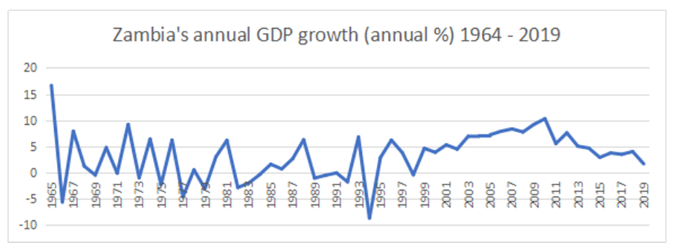 | Figure 2. Zambia's Annual GDP growth (1964-2019) |
As shown in Figure 2 above, Zambia has recorded an exceptional and exciting case beginning at independence in 1964 as a MIC (16.5% annual GDP growth rate in 1965) and subsequently declined to a low-income country for a long time before graduating to low-middle-income status. Typical of most developing countries, Zambia's economic growth was mainly input driven from the exploitation of physical and human capital resources.In 1964, 47% of Zambia's GDP was generated by mining, while agriculture (commercial and subsistence) accounted for only 11.5% and manufacturing for 6%. Therefore, although the economy benefited from mining, it is clear that the other economic sectors were still underdeveloped. Without economic diversification, the gains from mining alone would not lead to sustainable economic growth. Figure 2 above shows that the Country's GDP growth rate has remained consistent (3% average) with the lowest growth experienced in the late 1970s and mid-1990s. While the new government opted for a free market economy just after independence, it broke from its market-driven policies and opted for state control in the early 1970s. Instead of adopting structural transformation and economic diversification, the Zambian government adopted regulatory policies. During that period, economic growth remained unresponsive to the state intervention strategies until 1978 when the state acknowledged this approach's failure and the limited growth in the period 1977 – 1978. It was at this point that the government implemented Zambia's first Structural Adjustment Program (SAP).Zambia recorded its lowest economic growth in the 1990s. This was mainly due to the failed economic policies of the UNIP government. At that time, the MMD took over an unstable and contracting economy coupled with high poverty levels and inequality as well as a failing copper dominated export sector and a huge external debt. With government change, the MMD implemented the fourth SAP and focused on; macroeconomic stabilization, agricultural reforms, privatization of state assets and external liberalization. Although these reforms hoped to stimulate growth and diversify the economy, GDP growth remained stagnant at 0.2% throughout the 1990s. Despite the sustained economic growth in terms of GDP, there has been a marginal increase in GDP per capita income. The study has compared GDP per capita growth trends for Zambia to that of other countries. In particular, the average growth rates for Sub-Saharan Africa and the average for lower-middle-income countries in the world can be seen in Figure 3 below. 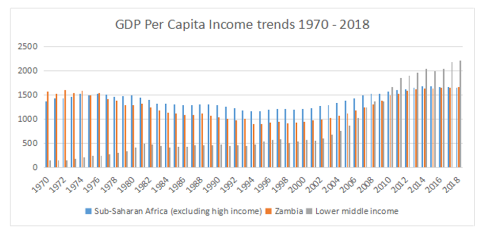 | Figure 3. Annual GDP growth Rate Zambia/ lower middle income countries (Source: Author Based on World Bank Data) |
When Figure 3 is analyzed, Zambia's GDP per capita growth rate was higher than the Sub-Saharan Africa average as well as that of lower-middle-income countries up until 1978. After this period, Zambia's GDP per capita dropped below the average in Sub-Saharan Africa until 2018.Despite attaining middle-income states in 2010, Zambia's GDP per capita growth rate is below the average for lower-middle-income countries in the world. Analyzing the graph, economic growth regressed in Sub-Saharan Africa in the period 1980 to 2000 and is only observed to pick up from 2008 onwards. During this period, the annual GDP growth rate for Sub-Saharan Africa reduced to 2.1% compared to 4.8% during the period 1960-1980. The reduction in growth resulted from the external shocks of oil price increases, declining terms of trade, and increased interest rates. Changes in Sector Contribution to GDPContrary to economic growth theories, non-agriculture related revenue accounted for Zambia's GDP's large share in the country's initial development process. According to Rostow (1956), a country goes through five development stages namely, (1) Traditional Society, (2) Preconditions to take off, (3) Take off, (4) Drive to maturity and (5) Age of high mass consumption.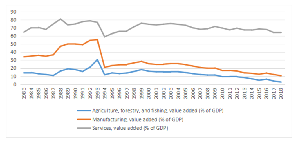 | Figure 4. Zambia sector contribution to GDP 1983 -2018 (Source: Author Based on World Bank Data) |
In the period 1983 to 2019, services and manufacturing sectors have maintained a larger percentage of Zambia's GDP. In terms of economic structure, it would imply that Zambia had already graduated from the Traditional Society and is now at Stage 2 (Preconditions for take-off). According to Rostow, at this stage, a country begins to develop manufacturing, and a more national/international, as opposed to regional, outlook. The stage is characterized by moderate per capita income growth, moderate structural change, increased share of non-agricultural labour and progressive infrastructure development. While services and industry seem to be on the right track, the regress in agriculture share to GDP is too fast, indicating an incomplete agricultural transformation.A further drop in agriculture share to GDP has far-reaching implications on poverty reduction and income inequality. It is also clear from the graph above that a reduction in agriculture of GDP has a direct impact on the secondary sectors (manufacturing and services). Therefore, agriculture is key to sustaining and increasing economic growth.Based on literature review, the MIT is caused by the changing role of factors that support growth in low-income countries that have reached middle-income status. More specifically, reliance on labour-intensive processes, imported technologies and foreign investment becomes less viable as growth pushes domestic prices and wages upward. It then becomes necessary to increase labor and capital productivity, facilitate rising total factor productivity, develop new technologies, and innovate. In Zambia, there is a need to boost productivity in the agriculture sector through improved technology and innovation. Research Question and Objective of the StudyThe rigorous review gives the following research question: What economic sectors affect Zambia's GDP per capita income level?ObjectiveTo establish the factors that affect Zambia's GDP per capita.
2. Methodology
In line with the literature review, we specify a model for assessing the variables that affect Zambia's GDP per capita income level. Thus, GDP per capita income, labour productivity, agriculture share to GDP, and manufacturing industry share to GDP were investigated. The model specification is inspired by a similar study conducted by Sevilay Konya et al in 2015.The study model will be: PCI represents per capita income level; M represents manufacturing share to GDP; L represents labor productivity; A represents agriculture's share to GDP. To ensure the model is technically sound, we perform a series of tests as follows; 1. Stationarity tests Typically, the first step in time series data modelling is to test for stationarity among the model variables. This is to ensure that the estimated relationships among the variables are not spurious. This study uses the Augmented Dicky Fuller (ADF) test, verified by Phillip Perron test.2. Determine the Optimal lag length (k) for the modelBefore testing for cointegration, we perform the optimal lag length selection test using all the criterion available in E-views 10 namely; Akaike Information Criterion (AIC), Schwarz Information Criterion (SC), Hannan-Quinn Information Criterion (HQ), adjusted R-squared and Final Prediction Error (FPE). In this study, the sequential modified LR test, Final prediction error and Hannan-Quinn information criterion will be used to determine the optimal lag selection.3. Johnsen Cointegration test Depending on the results of the cointegration test, we estimate either the VAR model or VECM. If the variables are integrated of order (1), we specify with (p) lags and estimate the VECM. If no cointegrations is found, we estimate the unrestricted VAR model. 4. Diagnostic testsDepending on the cointegration test results, diagnostic tests will be conducted before the actual causality tests are done. The following tests will be done on the modela. Autocorrelation test:b. Normality test:c. Stability test:5. Test for CausalityThe final step of the methodology will be to test for causality. Having subjected the study model to a series of tests outlined in steps 1 – 4, we conduct the Ward coefficient restriction test while the pairwise granger causality test will be performed to establish the direction of causality. DataNational and global economic data was used from various sources including the Zambia Central Statistical Office (CSO), the World Bank and FAO. Thes were the main sources of quantitative data. The data dates range from 1970 to 2019 and include annual data for the variables on the model.
3. Presentation of Findings
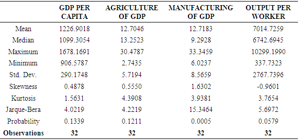
Descriptive Statistics Table 1 shows the descriptive statistics of all variables that were used to assess whether any causal relation exists GDP per capita, agriculture, manufacturing, and output per worker. The summary statistics show that only manufacturing as a share of GDP and Output per worker were not normally distributed because the probabilities associated with their respective Jarque-Bera test statistic of normality were less than 5%. The non-normality of these two variables does not affect the times series estimations but that of the model error term (Fox, 2015).Table 1. Variable Descriptive Statistics – Annual data (1970 – 2019)
 |
| |
|
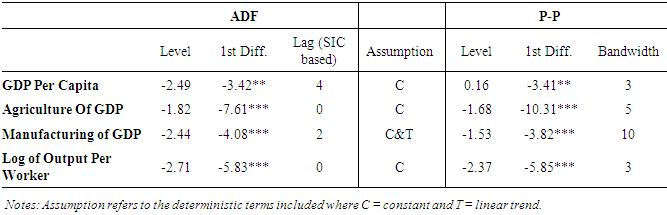
Unit Root The results for the unit root tests for the four variables of interest in this study are presented in Table 2. These results are confirmed by the ADF and backed by Phillip Perron tests of stationarity. Table 2. Unit Root Tests
 |
| |
|
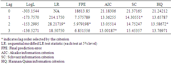
The asterisks (*), (**) and (***) imply significance at 10%, 5% and 1% levels respectively. The results show that all variables only become stationary at first difference as evidenced by their respective ADF and PP statistics whose P-values are all less than 5%. Hence, the null hypothesis that there is a presence of a unit root in the variables is only rejected for each variable at first difference. That is there is sufficient evidence suggesting all variables are now stationary at first difference implying they are integrated of order 1 i.e. I (1). To ascertain whether to use the VECM or VAR, Johansen cointegration test was conducted to determine the number of cointegrating equations. Optimal Lag SelectionBefore testing for cointegration, the optimal lag length selection test was done using all the criterion available in E-views 10 namely; Akaike Information Criterion (AIC), Schwarz Information Criterion (SC), Hannan-Quinn Information Criterion (HQ), Adjusted R-squared and Final Prediction Error (FPE). In this study, the Sequential Modified LR test, Final Prediction Error and Hannan-Quinn Information Criterion were used to determine the optimal lag selection. The criterion shows that the optimal lag in this model is 2 as shown in Table 3.Table 3. VAR Lag Order Selection Criteria
 |
| |
|
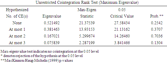
CointegrationHaving found that all the variables are integrated of order (1), we now carry out the Johansen cointegration test developed by Johansen (1988), below are results of the maximum eigenvalue test.Table 4. Johansen Cointegration Test
 |
| |
|
Based on the maximum eigenvalue statistic, the above results show no cointegrating relationship among variables at a 5% level of significance. Thus, the null hypothesis is that no cointegrating relationship is rejected because the eigenvalue statistic is greater than the critical value at 5%. Thus, the appropriate model is the Vector autoregressive model (VAR).
4. Diagnostic Test Result
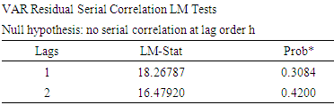
Serial Correlation TestThe serial correlation test was conducted using the Breusch-Godfrey LM test as in the Table 5. Since the probability values both at lag 1 and 2 are greater than 5%, we cannot reject the null hypothesis of no serial correlation in the model. Thus, the model has no serial correlation. Table 5. Autocorrelation Test
 |
| |
|
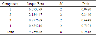
Normality TestTable 6 presents normality tests of the estimated Vector autoregressive Model (VAR) which was carried to test the normality of the model. Before any formal interpretations and policy implications can be made, the normality test needs to be done to ensure the model is not mis-specified, and that parameters are stable, unbiased, and consistent.Table 6. Normality Test
 |
| |
|
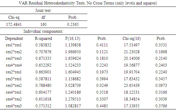
Based on the results presented in Table 6, the joint p-value of the joint Jarque-Bera statistic is greater than the 5%, so we have insufficient evidence to reject the null hypothesis that the residuals of the model are normally distributed. Hence, it can be concluded that the residuals are normally distributed. Heteroskedasticity TestThe results reveal that the joint P-value for Chi-square Statistic of the VAR Residual Heteroskedasticity Tests is greater than 0.05. Furthermore, all the p-values of the chi-square statistic for each individual component are greater than 5%. Table 7. Heteroskedasticity Test
 |
| |
|
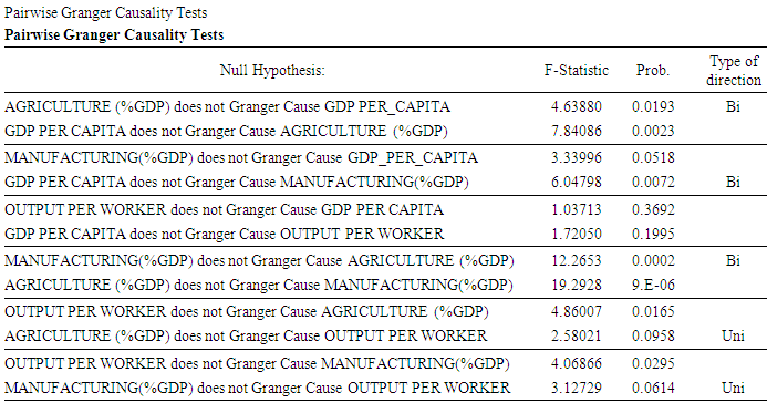
Therefore, we cannot reject the null hypothesis of no heteroscedasticity. Heteroscedasticity refers to data with unequal variability across a set of second, predictor variables. Data that shows heteroscedasticity gives biased coefficients.Tests for CausalityTo determine whether GDP per Capita was sensitive to own past changes, past changes in relative manufacturing as a share of GDP, agriculture as share of GDP and output per worker, granger causality tests were conducted using the Ward coefficient restriction test. In assessing the direction of causality, the pairwise granger causality test was used. The Granger causality test results are presented in Table 8 below.Table 8. Causality Test
 |
| |
|
Agriculture as a share of GDP granger causes GDP per capita and the converse also holds true. That the causality between GDP per capita and agriculture as a share of GDP per capita is bidirectional. The results from the table also shows that manufacturing as a share of GDP weekly granger causes GDP per capita, on the other hand, GDP per capita as a share of GDP strongly causes manufacturing as a share of GDP. Another bidirectional causality is between manufacturing as a share of GDP and agriculture as a share of GDP. That manufacturing as a share of GDP is sensitive to the changes in agriculture as a share of GDP and the opposite is true. Additionally, the results show that output per worker granger causes manufacturing as a share of GDP while manufacturing does not granger cause output per worker. That manufacturing as a share of GDP is sensitive to the changes of output per worker.The results from the table also reveal two unidirectional results. Output per worker does granger cause agriculture as a share of GDP but agriculture as a share of GDP does not granger cause output per worker. Furthermore, the results also show that output per worker does granger cause manufacturing as a share of GDP but manufacturing as a share of GDP does not cause output per worker at a 5% level of significance. The Wald test results for causality also show that only the first lagged GDP per capita granger values cause current GDP per capita at 5% level of significance. From the above result, two key bi-directional results are of interest based as follows;1. Agriculture share of GDP strong affects GDP per capita and the opposite is true2. Manufacturing as a share of GDP is sensitive to the changes in agriculture as a share of GDP and the opposite is trueWhile some causality has being found on the other variables, the causality relationships are not bi-directional. The following section discusses the implication of the two main findings after which conclusions will be drawn and recommendations given.
5. Discussion
Agriculture share of GDP strong affects GDP per capita and the opposite is trueIn line with the structural transformation of the economy, Zambia's GDP per capita is highly dependant on the share of agriculture to GDP. This result is consistent with the findings of various authors, Titus O. Awokuse, (2008), Joseph Phiri, et al. (2020). The authors agree that agriculture plays a vital role in developing countries' initial development process. It is the primary source of income for the rural population and a precondition for the growth of the secondary sectors such as industry and services. Despite its importance, Zambia's agricultures share of GDP has maintained a downward trend reducing from about 15% in 1983 to less than 3% in 2018. Based on this study's findings, poor agriculture performance will lead to reduced GDP per capita and low levels of economic growth. While the services and industry's GDP share has maintained an upward trend, there is a structural transitional problem as Zambia is shifting from resource-driven growth based on agriculture to growth based on advances in technology and innovation. This is confirmed by Gang Gong (2016). Gong identifies two main stages of economic development. He refers to the first stage as the period of digesting surplus labour and the second as the catching-up technology process. To transition from the first stage to the second, a country is expected to digest the surplus labour from the agriculture sector and in the process transform its production mode from being labour intencive to capital intencive. The inability to successfully transition from labour intensive to capital intensive mode of production is the reason for the MIT. The study's findings indicate that Zambia is at a great risk of being affected by the MIT due to this transitional challenge. Zambia's agriculture sector's current performance is an indication that the country has not fully transitioned from labour intencive to capital intencive modes of production. According to Gang Gong (2016), a country can only escape the MIT if the production mode successfully transforms from capital-intensive to knowledge-intensive. Manufacturing as a share of GDP is sensitive to the changes in agriculture as a share of GDP and the opposite is trueWhile no strong causality has been found between the manufacturing share of GDP and GDP per capita, manufacturing share of GDP has a strong influence on agriculture share of GDP which affects GDP per capita. These findings stress the importance of investing in both manufacturing and industry as the sectors mutually benefit each other. This is consistent with the findinds of Dan Su and Yang Yao (2018). They state that a decline in the manufacturing sector negatively affects an economy's service sector and noted that manufacturing provides an incentive for savings and can also accelerate the rate of technological progress. Qunhui Huang et al (2017), found that the increase in manufacturing share of GDP keep increasing as per capita income increases. They argue that manufacturing is key to escaping the MIT.In the case of Zambia, improvements in manufacturing can help to mechanize the agriculture sector and ultimately increase agriculture production. On the other side, improved agriculture output can provide the required raw material for industrial prosperity. In both cases, industry and agriculture are strongly linked as agriculture is the source of inputs needed in the agro related industry and utilizes other industrial inputs such as chemicals and farm equipment. In order to avoid de-industrialization, the government of Zambia should ensure adequate investment to support both agriculture and industrial development. Such investment should promote improved technology utilization and innovation.
6. Conclusions, Recommendations and Scope for Further Research
Consistent with the stages of growth theory and other studies reviewed in this paper, this study has shown that Zambia's GDP per capita is strongly affected by Agriculture's share to GDP. This indicates that Zambia is still transitioning from a labour intensive to a capital-intensive mode of production. This means that agriculture is still important to the structural transformation of the economy and is a precorser to the growth of the secondary sector. To get full benefits from agriculture, government intervention is required to stimulate a supportive industrial growth in order to provide the needed technology and services in agriculture. As confirmed by the granger causality results in the study, the manufacturing share of GDP is sentive to the changes in the share of agriculture to GDP. The continued drop in agriculture share to GDP may lead to di-industrialization and further a drop in the country's GDP per capita. Therefore, the solution to avoiding the MIT in Zambia lies in the agriculture and industrial sector.
7. Recommendations for Further Studies
Given that Zambia faces a transitional challenge, further studies could be conducted to establish how to catalyze the transition from a labour-intensive mode to a capital-intensive production mode.
References
| [1] | Abdulai, A., & Abdulai, A. (2017). Examining the impact of conservation agriculture on environmental efficiency among maize farmers in Zambia. Environment and Development Economics, 22(2), 177-201. doi:10.1017/S1355770X16000309. |
| [2] | Agenor, P.-R. (2016). Caught in the Middle?: The Economics of Middle-Income. Journal of Economic Surveys, 2. |
| [3] | Baillie, Richard T. 1996. "Long Memory Processes and Fractional Integration in Econometrics." Journal of Econometrics 73 (1): 5-59. |
| [4] | Baillie, Richard T. 1996. "Long Memory Processes and Fractional Integration in Econometrics." Journal of Econometrics 73 (1): 5-59. |
| [5] | Chirwa, T. G., & Odhiambo, N. M. (2015). The Dynamics of the Real Sector Growth in Zambia. Global Journal of Emerging Market Economies, 9. |
| [6] | Dieye, A. M. (26 de June de 2014). Devex. Obtenido de Devex: https://4m.cn/Vpf8h. |
| [7] | Felipe, J., U. Kumar, and R. Galope. 2017. Middle-Income Transition: Trap or Myth? Journal of the Asia Pacific Economy. |
| [8] | Hacker, J. (2004). Privatizing Risk without Privatizing the Welfare State: The Hidden Politics of Social Policy Retrenchment in the United States. The American Political Science Review, 98(2), 243-260. Retrieved January 10, 2021, from http://www.jstor.org/stable/4145310 ISSN 0165-1889, https://doi.org/10.1016/0165-1889(88)90041-3. |
| [9] | Kelvin Mulungu and John N. Ng'ombe 2017 Economies 2017, 5(2), 15; https://doi.org/10.3390/economies5020015. |
| [10] | Kharas, H. Kohli (2011). What Is the Middle Income Trap, Why do Countries Fall into It, and How Can It Be Avoided? Global Journal of Emerging Market Economies 3(3):, 281-289. |
| [11] | Kim, H. (1997) 'International diversification: effects on innovation and firm performance in product-diversified firms', Academy of Management Journal 40: 767-798. |
| [12] | Mattoo and Payton 2007 Services Trade and Development The Experience of Zambia Authors/Editors: Aaditya Mattoo , Lucy Payton https://doi.org/10.1596/978-0-8213-6849-7. |
| [13] | Ndulo and Mudenda 2010 Global Financial Crisis Discussion Series Paper 22: Zambia Phase Overseas Development Institute London, UK. |
| [14] | Qunhui Huang; Gang Liu; Jun He, Feitao Jiang; Yanghua Huang (2017), The middle-income trap and the manufacturing transformation of the people's republic of china (prc): asian experience and the prc's industrial policy orientation, ADBI Working Paper Series. |
| [15] | Rostow, W.W. (1960) The Process of Economic Growth. Oxford: Clarendon Press. |
| [16] | Sevilay Konya, Z. K. (2016). The Middle Income Trap: An assessment in terms of the Turkish economy. International Journal of Diplomacy and Economy, 4. |
| [17] | Solow (1956) The Quarterly Journal of Economics, Volume 70, Issue 1, February 1956, Pages 65-94, https://doi.org/10.2307/1884513. |
| [18] | Søren Johansen, 1988, Statistical analysis of cointegration vectors, Journal of Economic Dynamics and Control, Volume 12, Issues 2-3, Pages 231-254. |
| [19] | Takatoshi Ito (2017) Journal of International Money and Finance Volume 74, June 2017, Pages 232-257. |
| [20] | Zambia, MACO (Ministry of Agriculture and Cooperatives) 2004. National Agricultural Policy 2004-2015. MACO, Lusaka. |

 Abstract
 Reference
 Full-Text PDF
 Full-text HTML