Makaye Gongbé Blaise1, Gongbe Senouin C. Raissa2
1UFR SED, Alassane Ouattara University, Bouaké, Researcher at the Laboratory of Analysis and Modeling of Economic Policies (LAMPE), CRD, Alassane Ouattara University, Abidjan, Ivory Coast
2Project 100 Women Doctors for 2025 (CRDI Funding), of the Interuniversity Third Cycle Program (CIEREA-PTCI), Félix Houphouet Boigny University, Abidjan, Ivory Coast
Correspondence to: Makaye Gongbé Blaise, UFR SED, Alassane Ouattara University, Bouaké, Researcher at the Laboratory of Analysis and Modeling of Economic Policies (LAMPE), CRD, Alassane Ouattara University, Abidjan, Ivory Coast.
| Email: |  |
Copyright © 2021 The Author(s). Published by Scientific & Academic Publishing.
This work is licensed under the Creative Commons Attribution International License (CC BY).
http://creativecommons.org/licenses/by/4.0/

Abstract
This paper analyzes the individual effects of various fiscal instruments practiced in Côte d'Ivoire on national revenue. In a macro econometric model including the behavioral equations of economic agents submitted to taxation, and whose economic behavior has an impact on national revenue, we evaluated over the period 1996-2013, the effects of various taxes retained, on national revenue. The results show, on the one hand, that taxes on exports, value added tax, and household income tax had negative effects on national revenue during the study period with a relatively small effect for household income tax. On the other hand, taxes on imports and the tax on financial corporations have had positive effects on national revenue. As for the tax on non-financial corporations, its effects on national revenue are alternating but, generally positive.
Keywords:
Taxes, Economic growth, Macro econometric modelling
Cite this paper: Makaye Gongbé Blaise, Gongbe Senouin C. Raissa, Are There Good Taxes and Bad Taxes in Côte d'Ivoire Economy?, American Journal of Economics, Vol. 11 No. 1, 2021, pp. 1-9. doi: 10.5923/j.economics.20211101.01.
1. Introduction
While waiting for another alternative, tax revenues remain the main source of income for any government, for the achievement of its economic policy objectives of the magic square, the most important of which remains the growth of national income. But if the mobilization of tax revenues is not mastered, it may be incompatible with the development of economic activities. It is therefore worth considering the influence of fiscal policy on national income. This topic, both old and recurrent in the economic literature, is all the more useful in developing countries such as Côte d'Ivoire, given their low capacity to mobilize tax revenue.Since 2012, Côte d'Ivoire has achieved economic performance with an average growth of 8%. However, like most countries in sub-Saharan Africa, the public debt of Côte d'Ivoire has continued to grow and is estimated at 24.5% of GDP in 2017 against 23.1% of GDP. In 2016 (World Bank, 2018).This situation could be due to the budget deficits in the country in recent years. Indeed, even if it remains under control, Côte d'Ivoire's budget deficit increased from 4% of GDP in 2016 to 4.5% of GDP in 2017 (CAPEC, 2018). The recourse to debt to finance the economy is due to the weakness of the mobilization of internal resources. Government revenue in Côte d'Ivoire consists mainly of tax revenue and non-tax revenue. Tax revenue is the main source of government revenue, accounting for over 83% of total government revenue (Keho; 2010). This means that the repayment of the current debt of the Ivory Coast will be done mainly through the mobilization of fiscal revenue in the years to come.As regards the practical management of economic policy, the difficulty facing governments is therefore to find the combination of taxes that will not reduce national income, by distinguishing the most beneficial taxes from the most restrictive ones, so that debt repayment does not harm national income. Economic gains could therefore be obtained by modifying the tax structure if the effects of each tax instrument are known. Keho (2010) shows that the level of tax pressure is more damaging to growth than the structure of tax revenues. Hence the importance of carrying out more refined research that sheds light on the effect of each tax on national income. Knowledge of these different effects will therefore be a valuable source of information in the definition of fiscal policies. This is the aim of this paper, which attempts to capture the effects of the various taxes applied in Côte d'Ivoire on national income. In the rest of this work, section 2 briefly reviews the works on the subject. Section 3 presents the Ivorian tax structure, section 4 the model and statistical data. Section 5 presents the main findings, and section 6 a brief conclusion.
2. Literature Review
Theoretically, the relationship between taxes and national income is quite controversial.For some authors of classical obedience, the tax is a source of distortion and prevents the economy from reaching full employment. For Keynesians, on the contrary, taxes are a source of growth if good fiscal policy is implemented. The empirical link between tax structure and national income has been analyzed in several studies tending to show a relation between GDP (dependent variable) and independent variables such as the rate of productivity growth, total taxes, taxes on businesses, goods and services, imports and exports, etc...Bretschger (2010) and Padovano and Galli (2002) find a negative impact of corporate taxes on economic growth. Glomm and Ravikumar (1998) and Slemrod (2003) find that there is a positive correlation between taxes (on personal income, on company profits, VAT) and growth. Lee and Gordon (2005) find that raising taxes on companies leads to a low rate of GDP growth in the future.Using dynamic panel data over the period 2000-2012, Nantob (2014) analyzed the effects of the tax structure on growth in 47 developing countries. The results indicate that there is a non-linear relationship between tax revenue and economic growth, in particular, these taxes increase growth in the short run and this effect then increases over time as these taxes increase. Then there is a non-linear (U-shaped) relationship between taxes on income, profits and capital gains, taxes on international trade, and economic growth. Specifically, these taxes reduce short-term economic growth and these effects then diminish over time as these taxes increase.Chigbu and Njoku (2015) showed, for example, that there is a positive relationship between the independent variables, namely customs and excise duties, personal income taxes, taxes on petroleum profits and the variables dependent namely GDP, unemployment and inflation. However, the individual variables and the explanatory variables did not respectively contribute significantly to economic growth, to the reduction of unemployment and to inflation. As for Kosh et al (2005), they prove that the reduction in the tax burden has a strong impact on the level of economic growth, and also that the reduction in the direct tax burden has a low impact on the growth potential, compared to the indirect tax charge. They used the two-step modeling technique to control for unobservable business cycle variables. Regarding the Ivorian economy, Keho (2010) has shown, using a scaled-lag autoregressive model and an error correction model, the existence of long-term positive relationships between tax variables and gross domestic product. In the short term, however, he finds that certain types of taxes reduce economic growth in Côte d'Ivoire.
3. Distribution of the Different Types of Tax in Côte d’Ivoire
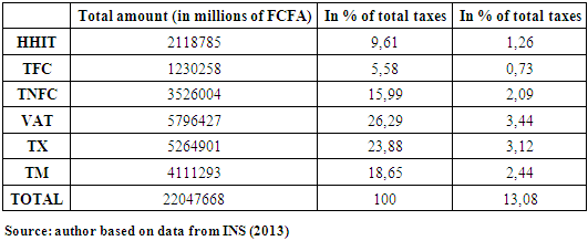
We show from the values recorded in Table 1, we show the share of the different types of major taxes applied in Côte d'Ivoire.Table 1. The share of each type of tax in the total amount of taxes and in that of real GDP
 |
| |
|
When we examine this table we find that the average tax pressure rate is 13.08%. This rate, in addition to being very low compared to the rates practiced in developed countries (40% and more) according to Besley and Person (2014), is low compared to that fixed by the WAEMU convergence criteria which is by 17%. We also note that the domestic taxes applied to households in particular the household income tax (HHIT) and the value added tax (VAT) contribute respectively on average to 35.9% to the total amount of taxes and to 4.7% to the amount of the GDP. As for domestic taxes on companies made up of tax on financial corporations (TFC) and tax on nonfinancial corporations (TNFC), they respectively account for 21.57% of total taxes and 2.82% of the value of GDP. Finally, the taxes applied to foreign trade, namely tax on import (TM)) and tax on export (TX), specifically contribute 42.53% and 5.7% of the total value of taxes and of the amount of GDP. In view of the information provided by Table 1, we can say that the taxes which occupy a preponderant place in the GDP are the taxes on foreign trade, then we have domestic taxes on households and finally domestic taxes on businesses.Here, as in most developing countries, tariffs are important, as Keho (2010) attests. Also for Perret et al (2016), in the early stages of development, a country has a more accentuated role of customs duties which could gradually decrease over time and be offset by additional revenue from VAT. The lower share recorded by domestic taxes applied to businesses is justified by the fact that the Côte d’Ivoire economy is characterized, like the underdeveloped countries, by a predominant informal sector. This has a strong impact on the fiscal pressure the taxpayers face in the formal sector. Thus, the low share of taxes on domestic businesses is largely justified by the low number of businesses taxed. As for domestic taxes on households, the highest amount is VAT. This significant share could be justified by the fact that VAT, a consumption tax, is paid by all economic agents without distinction; thus by its regressive character, it affects the poor as well as the rich. As for the household income tax, its low share is also due to the small size of households employed in the formal sector.
4. Model and Data
Most of the work analyzing the link between national income and taxation in the sub-region uses time series analyzes (MCE, ARDL), panels, and the DEA method. These article involve few equations, sometimes only one equation. As a result, we can find global relationships based on the average of the effects of one variable on another. Thus, it would also be interesting to analyze the question using a methodological approach involving several equations, which can help to better capture the complexity that the influence of the tax structure on the economy could take. And since taxes can modify the behavior of economic agents submitted to taxation, which in turn can influence GDP, we propose a model that can include all of these agents, such as grouped into institutional sectors by the national accounts, namely households, financial companies, non-financial corporations, the state, non-profit institutions and the rest of the world. This could allow more detailed results to be obtained, thus complementing existing work on the topic on study.
4.1. The Theoretical Model
To measure the effects of the various taxes on national income in Côte d'Ivoire, we use the Keynesian macroeconomic equilibrium which reflects the equilibrium on the market for goods and services, and which include all the institutional sectors submitted to taxation. This choice is motivated by the fact that taxes are supposed to have a distorting effect on the market for goods and services because taxes can modifying the behavior of economic agents grouped into institutional sectors. Subsequently, we introduce the various taxes that can upset the equilibrium on the market for goods and services in the original model.We start from the following Keynesian macroeconomic equilibrium in an open economy, on the market of goods and services: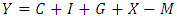 | (1) |
With: Y = national income, C = Private consumption, I = Private investment, G = Government expenditure, X = exports and M = importsBy setting that: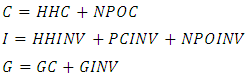 We obtain:
  | (2) |
With:  = Household consumption (constant),
  = Government consumption (constant),
  = Non-profit organisations consumption (constant),
  = Government investment (constant),
  = Private companies investment (constant),
  = Non-profit organisations investment (constant),
  = Household investment,
  = Exports (constant),
  = Imports (constant).In addition to the variables
  wich are theoretically exogenous, we assume on the one hand, that the variables,
  and
and  are exogenous. On the other hand, the variables
  and
and  are assumed to be endogenous because it is possible to predict their evolution. Thus, it is necessary to find the functional forms of the variables assumed to be endogenous in equation (2).The household consumption functionHousehold consumption is assumed to be a function of their disposable income, price level and value added tax. The household consumption function can thus be expressed as follows:
 With:
With:  = household disposable income (current),
  = Consumption price index, and
  = value added taxes (constant).By setting the following accounting identity:
 The household consumption function becomes:
 With:
With:  = Gross primary household income (current),
  = social benefits other than social transfers in kind received by households (current),
  = Other current transfers received by households (current),
  = Other current transfers paid by households (current),
  = household income tax (current),
  = social contributions paid by households (current)The function of private investmentWe assume that private investment is a function of public investment, credit to the economy, and corporate tax. The private investment function can thus be expressed by the following relation:
  1,
1,  With:
With:  = credit to the economy (current), and
  = corporation tax (current)By setting that:
  we obtain:
 With:
With:  = taxes on financial corporations (current), and
 = taxes on non-financial corporations (current)The export functionExports are assumed to be a function of the terms of trade and export taxes. The export function can thus take the following form:
 With:
With:  = term of trade and
  = export taxes (constant)The import functionImports are assumed to be a function of the terms of trade and import taxes. The import function can thus be presented in the following form:
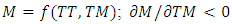 With:
With:  = import taxes (constant)Finally, the equilibrium on the market for goods and services (2) becomes:
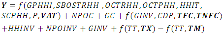 | (3) |
Thus, we obtain a model (3) which will be transformed into a system in the next sub-section. The change in a tax variables in bold letters on right hand side will result in change in national income Y represented by real GDP.
4.2. The Empirical Model
The point here is to proceed with the specification of an empirical form of Keynesian macroeconomic equilibrium from the previous subsection. Following the example of Klein and Goldberger (1955), we give econometric specifications to the endogenous variables of the previous model. This makes it possible to obtain a macro econometric model composed of accounting identities and econometric equations. After several estimates, the outputs of which were compared, the specifications below were adopted. Note that dummies were used to capture the election year and the post-election crisis. After these specifications, we obtain the system below, a macro econometric model, comprising 29 variables including 7 endogenous and 22 exogenous. Note that real gross domestic product has been used as a proxy for national income, and gross fixed capital formation as a proxy for investment.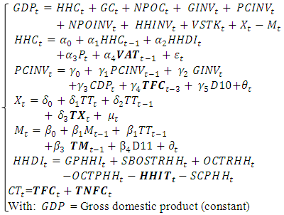 In its empirical form, we can see the lagged values of the household consumption because of the ratchet effect. According to this theory, the household present consumption depends on its passed values. The use of the lagged value allow to take into account the omitted variables because the lagged values contain the past determinants of the endogenous variable. The presence of the lagged value reduces the autocorrelation problem.We add the lagged value of PCINV in PCINV equation because we suppose that an investment started the last year can end this year, so the amount spend this year for an investment can be related to the one spend last year for the same investment. So it is important to take into account the lagged values of investment.The use of the lagged value of the imports allow to take into account the omitted variables and to reduce the autocorrelation problem.We suppose the exports depend on the present and the past terms of trade. The cocoa is produced two time in a year (beginning and the end of each year). The first harvest depends on the terms of trade of the past year, and the second harvest depends on the terms of trade at the beginning of the current year. After estimating the coefficients econometric equations, this model was solved by iteration in Eviews, using a solver, to determine a dynamic economic equilibrium, which will be call the baseline solution. Then, using simulations, we disturb this baseline equilibrium by modifying the tax variables of the model. This allow to catch the individual effects of the six taxes chosen, namely,
  and
and  , on real GDP over the study period.The data come from the national accounts provided by the INS (Tables of make and uses (TRE), tables of integrated economic accounts (TCEI)), except the exchange rate, price index, and credit to the economy that come from Word Development Indicator. Data from tables of resources and uses are at constant price, and data from tables of integrated economic accounts are at current price.All these data cover the period 1996-2013. Period for which all variables are covered by the national accounts. In fact, tables of resources and uses are available with a delay of five years as it can be seen in many African countries, and tables of integrated economic accounts take more time than Tables of resources and uses. Moreover, when working a model involving identities it is preferable to use data from the same source to conserve the equilibrium of those identities. That’s why data are limited on 2013.
5. Results and Discussion
The starting point of the use of a model consist of making the historical simulation, called the baseline scenario (Almon, 2017). The computed values of the GDP by the baseline scenario is compared to the actual values of GDP. This comparison make it possible to appreciate the overall goodness of fit of the entire model. The difference between the baseline scenario GDP values and the actual GDP values represents the model errors. The graph 6 making the comparison of baseline GDP values with actual GDP values is shown in appendix A2. It shows that the tow values of GDP are close. So the macro econometric model used has an appreciable power to forecast GDP.The coefficients obtained after estimation of the econometric equations of the model and their endogenous variables graphs which make it possible to assess the goodness of fit of these coefficients, are also provided in appendices A1. The results show that the baseline values of endogenous variables are close to their actual values.
5.1. Description of Scenarios
For the resolution of the model, we used the Broyden solver, with a tolerance of 10-8 for convergence and a maximum number of 5000 iterations. Note that we found similar results using the Gauss-Seidel and Newton solvers. The type of simulation used is stochastic simulation.In order to eliminate the model prediction errors in the simulations, the results of all scenarios will be compared to the results of the baseline scenario. Thus, any change in GDP values will be attributable to the changes of tax variables values. In each scenario, we set to zero a given fiscal variable values, then we run the model, and then compare the GDP values for this scenario to the baseline GDP values. This allows us to observe what the national income would have been if this tax had not been applied by the government during the period of the study.If the scenario GDP values are lower than the baseline GDP values (the values of GDP when this tax was applied), then we can conclude that this tax had positive effect on GDP. Otherwise, where the scenario GDP values are greater than the baseline GDP values, we conclude that the tax considered had a negative effect on the GDP over the study period. Thus:- In scenario 1, we set to zero the household income tax (HHIT) values over the study period;- In scenario 2, we set to zero the financial corporation tax (TFC) values over the study period;- In scenario 3, we set to zero the tax on non-financial corporations (TNFC) values over the study period;- In scenario 4, we set to zero the import taxes (MT) values over the study period;- In scenario 5, we set to zero the value added tax (VAT) values over the study period;- In scenario 6, we set to zero the taxes on exports (TX) values over the study period.
5.2. Scenario Results
The result of each scenario is presented in appendix A3. Graph 1 presents the synthesis of the results of the six scenarios mentioned above. The gaps representing the effects of each tax on GDP are obtained by the following calculation:
 With
With  difference between the GDP value in the baseline scenario and the GDP value in scenario i for a year t;
  GDP values from the baseline scenario for year t; and
  = the GDP value from the scenario i for year t.
 represents for each scenario, the effect of the relevant tax on GDP for each year over the study period.If
  then the taxes concerned have a positive effect on GDP. If
  then the taxes concerned have a negative effect on GDP. If
  then the taxes concerned have no effect on GDP;In graph 1, we compare the differences between the GDP values of each scenario (scenario 1 to 6) and the GDP values of the baseline scenario. This allows us to capture the individual dynamic effects of tax variables on the GDP over the study period.
 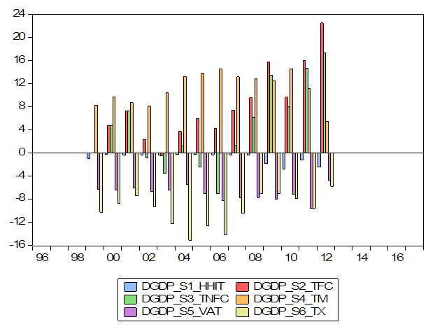 | Graph 1. Effects of fiscal variables as% of baseline GDP (Source: authors computations in Eviews) |
Graph 1 reveals the following information:First, the household income tax, the value added tax, and the export taxes have a negative effects on real GDP over the study period. This negative impact is higher for taxes on exports with an average loss of 9.8% of GDP. The VAT comes second, with an average loss of 6.9% of GDP, and the household income tax brings up the rear with an average loss of 0.8% in GDP.The results concerning export taxes agree with the findings of Bonjean and Chambas (1995). Indeed, export taxes having effects on export prices tend to discourage the production of agricultural goods, which is damaging for a country with primary specialization like Côte d’Ivoire. The negative effect of VAT obtained in this research contrasts with the long-term results obtained by Moussavou (2017) and Keho (2010), but in line with the short-term results of Keho (2010). Regarding the household income tax (HHIT), the result is in line with that obtained by Moussavou (2017) who points to its negative effect on the purchasing power of households.Then, import taxes and financial corporations tax have a positive effect over the study period. This positive effect is stronger for taxes on imports which come first with an average gain of 8% of GDP, and followed by the financial corporation tax with an average gain of 7.8% of GDP. Finally, the tax on non-financial corporations has an alternating effect over the study period, but generally positive with an average gain of 4.3% of GDP. Thus, the effect of the TNFC is positive from 1999 to 2001, negative from 2002 to 2006, positive from 2007 to 2013, with a gain of 10.2% of the GDP.
6. Conclusions
This paper analyzes the individual effects of various fiscal instruments practiced in Côte d'Ivoire on national revenue. Unlike previous work on the issue in the West Africa, which regresses GDP on fiscal variables, this paper adopts another approach bringing together in a macro econometric model, the behavioral equations of economic agents, who are submitted to taxation, and whose behaviors can affect GDP. Thus, using simulations, we computed over the period 1996-2013, the effects of the 6 major of taxes applied in Côte d’Ivoire, on gross domestic product. The results show, on the one hand, that taxes on exports, value added tax, and household income tax had negative effects on national income during the study period with a relatively small effect for household income tax. On the other hand, taxes on imports and the tax on financial corporations have had positive effects on national income. As for the tax on non-financial corporations, its effects on national income are alternating but, generally positive. In view of these results, policy-makers should favor tax instruments that are beneficial to national income, over restrictive instruments.
Appendices
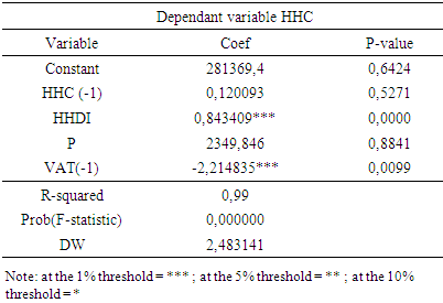
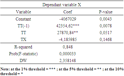
A 1: Results of the estimations of the model equationsWe present the coefficients obtained after estimating the econometric equations contained in the model. All the estimates have relatively acceptable. The graphs compare the values calculated by the baseline scenario, actual values available in the national accounts. This makes it possible to assess the goodness of fit of the estimated coefficients: the more the two graphs are close, the more acceptable the estimated coefficients are. In the case of a macro econometric model, the acceptance of coefficients depends more on how the model fit, than the econometrical properties that can always discussed.For example, for the consumption equation, the graph shows that the computed baseline values and actuals values of household consumption are relatively close. This shows that the coefficients of the household consumption equation are acceptable, even if they don’t satisfy all the econometric property. It is the same for all the other estimated equations of the model.Table 2. Estimate of the household consumption equation
 |
| |
|
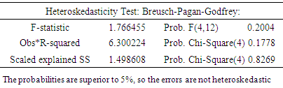
The Durbin Watson statistic = 2,48 lead to think about a problem of autocorrelation. We then do an autocorrelation test as provided in tables 3.Table 3. Autocorrelation test for HHC equation
 |
| |
|
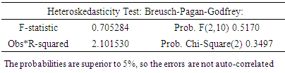
Table 4. Heteroskedasticity test for HHC equation
 |
| |
|
 | Graph 2. Predicted consumption and historical consumption (Source: authors computations in Eviews) |
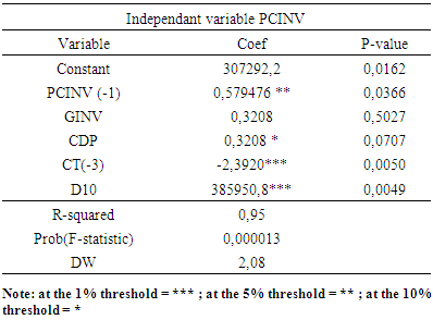
Table 5. Estimate of the private investment equation
 |
| |
|
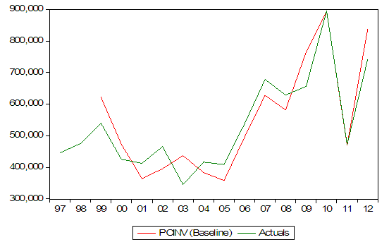 | Graph 3. Predicted private investment and historical private investment (Source: authors computations in Eviews) |
Table 6. Estimation of the exports equation
 |
| |
|
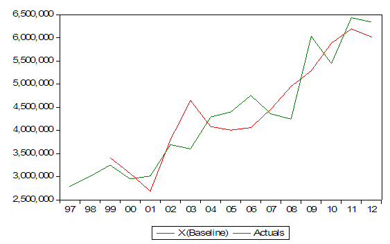 | Graph 4. Calculated exports and historical exports (Source: authors computations in Eviews) |
Table 7. Estimation of the imports equation
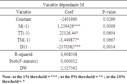 |
| |
|
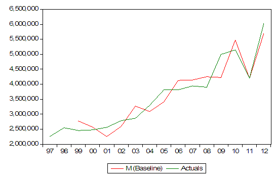 | Graph 5. Predicted imports and historical imports (Source: authors computations in Eviews) |
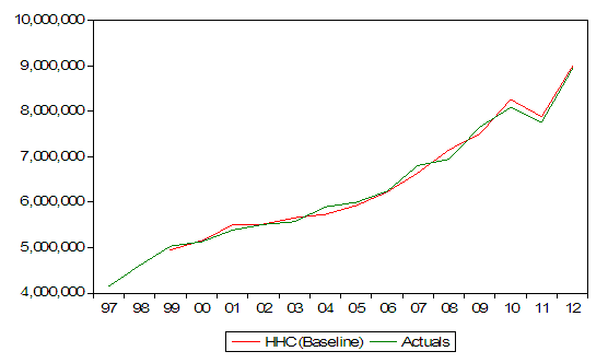
A 2: Model adjustmentThe graph 6 make the comparison of baseline GDP values with actual GDP values. 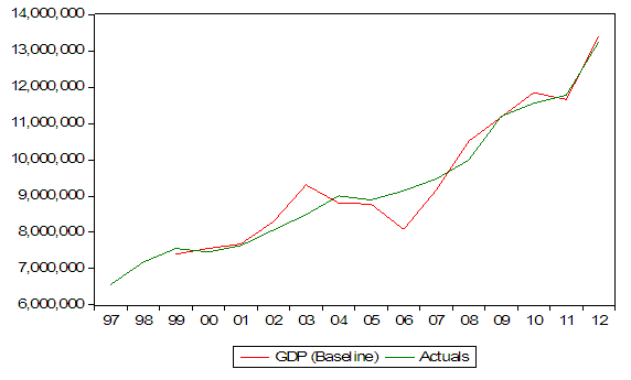 | Graph 6. Result of the baseline scenario: calculated GDP against historical GDP (Source: authors computations in Eviews) |
Graph 6 shows that the curves of the baseline GDP and the actual GDP provided by the national accounts are close. The model then has an acceptable predictive power of GDP. It can therefore be used to analyze the effects of different tax policy variables on economic GDP in Côte d'Ivoire over the study period.A3: results of the scenarios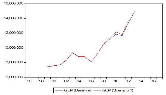 | Graph 7. Result of scenario 1 (HHIT) (Source: authors computations in Eviews) |
According to Figure 7, the scenario GDP is above the baseline GDP, so the household income tax resulted in growth losses over the study period.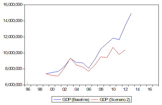 | Graph 8. Result of scenario 2 (TFC) (Source: authors computations in Eviews) |
Figure 8 shows that scenario GDP is lower than baseline GDP, so the financial corporation tax led to growth gains over the study period.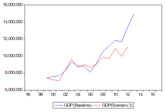 | Graph 9. Result of scenario 3 (TNFC) (Source: authors computations in Eviews) |
According to graph 9, from 1999 to 2001 the value of the GDP of scenario 3 is lower than that of the baseline GDP, over this period the TNFC had a positive influence on the GDP, and then from 2002 to 2006 the baseline GDP had a low value compared to that of the scenario GDP. Here the TNFC had a negative effect on the GDP, finally from 2007 to 2013, the baseline GDP is higher than the GDP of the scenario, so the TNFC therefore had a positive impact on GDP.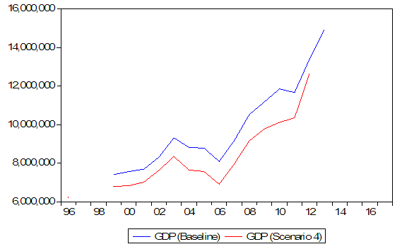 | Graph 10. Result of scenario 4 (TM) (Source: authors computations in Eviews) |
On graph 10, we see that the value of the scenario GDP is lower than that of the baseline GDP. So import taxes have been beneficial for economic growth over the period.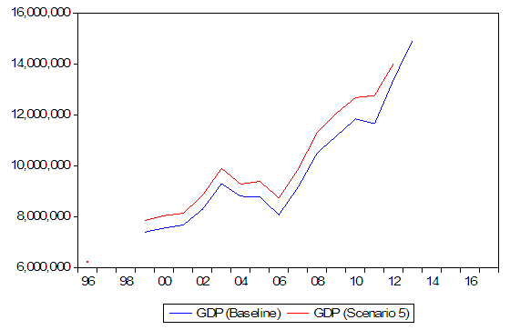 | Graph 11. Result of scenario 5 (VAT) (Source: authors computations in Eviews) |
According to graph 11, we find that in general over the period of analysis the baseline GDP is lower than the GDP of the scenario considered. Therefore, the VAT negatively influenced economic growth over the study period.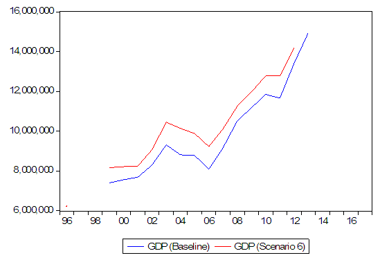 | Graph 12. Result of scenario 6 (TX) (Source: authors computations in eviews) |
On graph 12, we see that the value of the GDP of the scenario considered is higher than the value of the GDP of the baseline scenario. So, export taxes also had a negative impact on GDP over the study period.
Note
1. Theoretically, the derivative of private investment in relation to public investment can be positive or negative or zero, depending on whether there is a knock-on effect of public investment on private investment or crowding out or neutrality effect. In the case of Côte d'Ivoire, we assume that we are at a stage of development where public investment is still essential for the development of private activity, given the inadequacy of infrastructure.
References
| [1] | Almon (2017). The Craft of Economic Modeling. Third, Enlarged Edition. July 16. |
| [2] | Bonjean, C. and Chambas, G. (1995). Taxe foncière, taxe à l’exportation: l’expérience vietnamienne est-elle transposable en Afrique? Tiers monde, 36(144), 1995 pp.725-745. |
| [3] | Besley and Person (2014). Why Do Developing Countries Tax So Little?, Journal of Economic Perspectives, Volume 28, Number 4, Pages 99–120. |
| [4] | Bretschger, L. 2010. Taxes, mobile capital, and economic dynamics in a globalizing world. Journal of Macroeconomics, no. 32, pp. 594-605. |
| [5] | Chigbu, E.E., and Njoku, C. (2015). Taxation and Nigerian Economy: 1994-2012. Management Studies and Economic Systems (MSES), 2(2), pp. 111-128. |
| [6] | Glomm, G. and B. Ravikumar. 1998. “Taxes Government Spending on Education and Growth”, Review of Economic Dynamics, no. 1, pp. 306–325. |
| [7] | INS (2013), Institut National de la Statistique. http://www.ins.ci/n/. |
| [8] | Keho, Y. (2010a). Effets macroéconomiques de la politique fiscale en Côte d’Ivoire. Politique Economique et Développement, CAPEC-CIRES, Abidjan, Côte d’Ivoire. |
| [9] | Keho, Y. (2010b). Détermination d’une structure fiscale optimale des recettes fiscales en Côte d’Ivoire. Politique Economique et Développement, CAPEC-CIRES, Abidjan, Côte d’Ivoire. |
| [10] | Klein and Goldberger (1955). An Econometric Model of the United States (1929-1952). Amsterdam: North-Holland. |
| [11] | Kosh, S.F. and Al (2005). Economic growth and the structure of taxes in South Africa: 1960-2002. South African Journal of Economics, 73(2), pp.190-210. |
| [12] | Lee, Y. and Gordon, R. (2005). Tax structure and economic growth, journal of public economics, 89 (5-6), pp. 1027-1043. |
| [13] | Moussavou, F. (2017). Impact des structures fiscales sur la croissance économique au Congo Brazzaville. European Scientific Journal, 13(34), pp.163-185. |
| [14] | NANTOB (2014). Taxes and Economic Growth in Developing Countries: A Dynamic Panel Approach. MPRA Paper No. 61346. |
| [15] | Perret, S. and Al. (2016). Atteindre l’émergence : les défis fiscaux de la Côte d’Ivoire. Document de travail de l’OCDE sur la fiscalité, No.25, édition OCDE, Paris. |
| [16] | Padovano F. et E. Galli. 2002. Comparing the Growth Effects of Marginal vs. Average Tax Rates and Progressivity. European Journal of Political Economy, no. 18, pp. 529-544, 2002. |
| [17] | Slemrod, L. 2003. The Truth About Taxes and Economic Growth. Challenge, vol. 46, no. 1, 2003, pp. 5–14. JSTOR. |

 Abstract
 Reference
 Full-Text PDF
 Full-text HTML