1. Introduction

Many people have tried to explain the relationship between education expenditure and income inequality in some countries/regions in different ways. However, the outcomes are mixed. Some economists agree with the view that countries with more expenditure on education are associated with falling inequality. Glomm and Ravi Kumar (1992) [5] develop a model where there are two types of education system viz., private and public education system and people can choose one of them. They argue that income inequality is not declined under the private education system but unambiguously declines under the public education system. Schultz (1963) [15] argues that if the government is strengthening to increase support for public education income inequality will reduce. In the existing literature, some theoretical models give the inverse relationship between public education and income inequality. Saint Paul & Verdier (1992) [14], Eckstein & Zilcha (1994) [2] and Zhang (1996) [19] develop models where they argue that government should give continuous support to public education for reducing the level of income inequality over time. Sylwester (2000) [17] develops a model where public education can lower the level of income inequality if agents have sufficient resources to forgo income and attend school. If there is a variation in access to education, then increasing public education expenditure can cause the distribution of income to become more skewed since the poor are taxed for revenue but do not enjoy the benefits of the public education system. Ashen Felter and Rouse (2000) [1] believe that the school is a proper place to increase the skills and hence incomes of individuals. As a result, educational policies have the potential to decrease income inequalities. Heckman (2005) [6] states that human capital ultimately determines wealth. Fostering access to education will reduce inequality in the long run. Sylwester (2002) [18] suggests that for education expenditure may be an important factor for reducing income inequality along with other measurable factors. Kayet and Mondal (2016a) [8] prove that public education expenditure can help to reduce food inequality in rural India. On the other hand, some economists are not agreeing with this view. Although many countries allocate more resources to public education the degree of income inequality does not reduce, Fields (1980) [3]. Ram (1989) [13] examines many theoretical and empirical works and concludes that there is not a strong relationship between increasing education expenditure and lowering income inequality. In the face of these contradictory views, we are interested to find out the impact of public education expenditure¹ at different levels² (expenditure on elementary, secondary, and higher-level) on inequality measured by different measures (absolute, relative and index) in India.

However, two vital questions may arise. The first one is how education (especially education expenditure) do related to income inequality. Education has great strength for improving human development, accelerating social transformation, reducing economic inequalities, and achieving economic development. Education has a positive externality. An educated person gives many new ideas/technologies to society about how best to produce goods and services. If people accept these ideas then they can produce maximum output subject to minimum cost. The ideas are external benefits of education. Imagine a society; where there is a high demand for labourers especially, efficient labourers (literate labourers) create high wages for those having an education. Consequently, those who are inefficient (illiterate), generally receive much lower wages leading to higher inequality. Thus, equality in access to education leads to a decrease in income inequality. The second one is if they are related then why do we consider education expenditure as an explanatory variable or exogenous variable or predetermined variable and inequality as explained variable or endogenous variable or jointly determined variable. This is because public education expenditure is a policy variable as the government takes a policy for allocating the resources for public education in the budget and inequality is an effect variable. A policy variable should consider as an exogenous or predetermined variable and an effect variable should always consider an endogenous variable.

However, using panel data of 15 major states of India from 1983 to 2012 and by considering different types of inequality measures (an absolute measure of inequality, a relative measure of inequality, and an index measure of inequality) this paper examines whether public education expenditure at different levels (elementary, secondary, and higher) can reduce inequality in India or not.

2. The Debate between Relative and Absolute Inequality

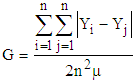
By economic inequality in a region/country, we mean the absence of equality in the distribution of economic variables like income, expenditure, wealth, etc. among the individuals/households in that region/country. Economic inequality especially, income inequality occurs due to the existence of disproportionate distribution of total national income among households whereby the share going to the rich persons in a country is far greater than that going to the poorer persons. This is largely due to differences for income derived from ownership of property and to a lesser extent the result of differences in earned income. Inequality can be measured by a relative measure of inequality and an absolute measure of inequality in different families of inequality measures. Economic inequality for India and its major states can be estimated only for expenditure and not normally for any other economic variable because NSSO collects household data only for the expenditure of the sample households and not for income or wealth. NSSO itself estimates inequality for India and its states through Gini coefficients (Gini, 1936 [4]) and Lorenz curves (Lorenz, 1905 [12]) and we all use those estimates for such purpose. We also use the raw data published by NSSO and have our estimates. The question of own estimation arises because we do not have satisfaction from these two measures. Thus, a question is how good and how much sufficient are these measures in inequality estimation? We feel that they are not sufficiently good – though they are still treated as better than other competing measures.

If Y₁, Y₂, …, Y_n are income levels of n individuals of a region/country in non-decreasing order with mean income then Gini coefficient for income distribution of this population is given by . Some academicians prefer to express the Gini coefficient as .

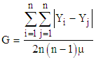It is a quantitative measure, a singular measure, an additive measure, a relative (as opposed to absolute) measure – relative to mean income and is a unit-free measure. For infinite population it is an index measure, its value lying between 0 and 1 – relative in another sense – relative to maximum possible absolute or relative value of inequality. On the other hand, the Lorenz curve is given by the locus of percentage income appropriations by percentage cumulative populations having income in the non-decreasing order. It is plural (as opposed to singular) measure, a qualitative measure, a relative (as opposed to absolute) measure, a unit-free measure. It is also an index measure for the infinite population.

Gini coefficient is equal to the Lorenz ratio. They use the same principle of inequality measurement. Both of them are relative measures. Both of them are unit free measures. Both of them are index measures for an infinite population. Lorenz curve is the graphical or plural counter-part of the Gini coefficient. They belong to the same family. Let us call the family the Lorenz-Gini family.

Now come to the question of how good or how logical this family is in inequality measurement. To be good it should satisfy some basic requirements/principles of inequality measure. Both Gini coefficient and Lorenz Curve satisfy the ‘principle of income transfer – the Pigou-Dalton principle’, ‘principle of proportionate additions to incomes’, ‘principle of additions to incomes’, and ‘principle of additions to persons’. Also, they approximately but not exactly satisfy the ‘principle of proportionate additions to persons’. But both the Gini and the Lorenz Curve fail to satisfy the ‘principle of equal additions to incomes’ and Gini fails to satisfy the ‘principle of decomposition by subgroups’ and the ‘principle of decomposition by components of incomes’.

Actually, inequality can be viewed both in absolute and relative senses. In the Lorenz-Gini family the absolute measure of inequality is 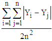. It is the pure per capita inequality and satisfies the ‘Principle of proportionate additions to persons’ and the ‘Principle of equal additions to incomes’. An absolute measure of inequality is not unit free and so inequality comparison across countries using different units of measuring income or over time in the same country with inflationary conditions becomes inconvenient. An absolute measure of inequality of this type has a fixed lower bound at 0 but its upper bound is not fixed. It is given by when all income is enjoying by a single person. For this reason, also an absolute measure of inequality is inconvenient for inequality comparison. It is also inconvenient for inequality comparison as it fails to compare inequality relative to mean income.

In this family the relative measure of inequality is . This is the Gini coefficient of the first type. It is the measure of inequality per capita and per rupee of mean income and satisfies the ‘Principle of proportionate additions to persons’ and the ‘Principle of proportionate additions to incomes’. A relative measure of inequality is unit free and so inequality comparison across countries using different units of measuring income or over time in the same country with inflationary conditions becomes convenient. It is also convenient for inequality comparison as it compares inequality relative to mean income. A relative measure of inequality of this type has a fixed lower bound at 0 but its upper bound is not fixed. It is given by when all income is enjoyed by a single person.

Kolm (1976) [10] has well taken up this debate between absolute and relative inequality. He has believed that inequalities can measure by both ways and the researchers in this field have used both of them. He has tried to define a relative measure of inequality as a ‘rightist’ measure of inequality as the richer section of the community or the capitalist class or their union prefers to accept it when income increases (by the equal amount or by equal proportion) and an absolute measure of inequality as ‘leftist’ measure of inequality as the poorer section of the community or the labour class or the labour union prefers to accept it when income increases.

He writes:

“In May 1968 in France, radical students triggered a student upheaveal which induced a workers’ general strike. All this was ended by the Grenelle agreements which decreed a 13% increase in all payrolls. Thus, laborers earning 80 pounds a month received 10 pounds more, whereas executives who already earned 800 pounds a month received 100 pounds more. The Radicals felt bitter and cheated; in their view, this widely increased incomes inequality. But this would have left unchanged an inequality index.”

“And I have found many people who feel that it is an equal absolute increase in all incomes which does not augment inequality, whereas an equiproportional increase makes income distribution less equal or more unequal – and these were people of moderate views. When all incomes are multiplied by the same number, whereas a relative measure of inequality does not change, an absolute measure of inequality is multiplied by this number. Therefore, if we study variations of an absolute measure of inequality over time in an inflationary country, we must use real incomes, discounted for inflation; or if we make international comparisons, we must use the correct exchange rates. This need not be done if we use a relative measure of inequality. Anyway, convenience could not be an alibi for endorsing injustice.”

However, viewing relative measure of inequality as ‘rightist’ and absolute measure of inequality as ‘leftist’ is not completely true, because when income falls (by the equal amount or by equal proportion) the richer section of the community or the capitalist class or their union prefers to accept an absolute measure of inequality and the poorer section of the community or the labour class or the labour union prefers to accept a relative measure. Anyway, these are two well-accepted views and Kolm himself was convinced of both the views. He has preferred to develop a ‘centrist’ view of inequality in between the two.

We are also actually convinced of both the views and probably like Kolm we also want to have a centrist view in between the absolute and relative views. We do not want that inequality remains constant with equal additions to incomes; rather we want that inequality fall. Similarly, we also do not want that inequality remains constant with proportionate additions to incomes; rather we want that inequality increase.

Thus, to have a complete view of inequality, we should have a plural view, it should be measured in both ways – absolute and relative. This may lead to a conflicting conclusion in both inter-temporal and inter-state comparisons. If we want to avoid this conflict and try to develop a singular measure, a centrist measure, we shall be in trouble once again because it is difficult to determine the relative weights of absolute and relative inequalities. We shall not go for that, rather we shall present them separately.

3. Database and Methodology

The sample consists of a cross-section of 15 major states of India. The sample period begins in 1983 and ends in 2011-2012. The raw data of household consumption expenditures are collected from a different quinquennial survey of consumption expenditures published by NSSO from 1983 to 2011-12 to have our estimation. The Gini coefficient and the coefficient of variation are considered to measure the relative inequality in the Lorenz-Gini family and SD-CV family respectively and the CV-index is used to measure the index of inequality in SD-CV family. The absolute Gini and the standard deviation are considered to measure the absolute inequality in the Lorenz-Gini family and SD-CV family respectively.

The raw data of education expenditure at different levels are collected from the Analysis of Budget Expenditure on education in different years published by the Ministry of Human Resource Development (MHRD). Per capita public expenditure on education at different levels is measured by rupees and is obtained from total public expenditure on education at different levels dividing by total population.

Expenditure on education has partial effects on economic inequality. Economic inequality depends on some socio-economic, demographic, political and other variables, Kayet and Mondal (2016b) [9], Kaasa (2003) [7], Sylwester (2002) [18]. The growth rate of output is considered to be an important factor in explaining income inequality. Kuznets (1955) [11] proposes by the inverted-U hypothesis that, with growth in per capita income, inequality rises initially but after some time, it reaches the maximum point and then returns to the original level. The population is an important demographic factor for explaining inequality. It affects inequality directly. The more the population of a state/country more will be the inequality. However, it is inversely related to the index of inequality in the SD-CV family measured by CV-index as, CV has to be divided by to have CV-index. Monthly per capita expenditure (MPCE) and work participation rate (WPR) are two important macroeconomic determinants for explaining economic growth. There is a direct relationship between MPCE and WPR and, economic growth. Rise (fall) in MPCE and WPR is an important cause for rising (falling) the economic growth. Theoretically, there is an inverse relationship between economic growth and equity. If economic growth rise (fall), equity will fall (rise), which means economic inequality will rise (fall). Thus, there is a direct relationship between economic growth and economic inequality. Hence, there is a positive relation between MPCE and WPR, and inequality. We have the raw data of MPCE for rural and urban areas from the different quinquennial survey report of consumption expenditure published by the National Sample Survey Orgnisation (NSSO). The raw data of WPR are collected from the different quinquennial survey reports of employment and unemployment published by the National Sample Survey Orgnisation (NSSO) for rural and urban areas.

3.1. Tools for Adjustment of Variables

Dependent Variable:

Different types of combined inequalities³ (relative inequality, index of inequality and absolute inequality) are taken into consideration for empirical estimation in this work.

Explanatory Variables:

1. Total public expenditure on education is divided into three levels viz., public expenditure on the elementary level, public expenditure on the secondary level and public expenditure on the higher level.

2. By taking into consideration the raw data of population from different census reports and with the help of these raw data we estimate the population in India and its major states by Lagrangian non-linear interpolation method as per need.

3. The annual compound growth rate of output is calculated by the formula;

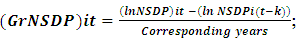Where, NSDP denotes net state domestic product, i denotes the cross-section of states, t denotes current period, k denotes previous period.

4. The combined monthly per capita consumption expenditure (CMPCE) is obtained from the weighted average of rural MPCE and urban MPCE and is calculated by the formula;

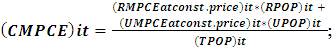Where, RMPCE denotes rural monthly per capita consumption expenditure, UMPCE denotes urban monthly per capita consumption expenditure, RPOP denotes rural population, UPOP denotes urban population, TPOP denotes total population, i denote the cross-section of states and t denotes current period.

5. The combined work participation rate (CWPR) is obtained from the weighted average of rural WPR and urban WPR and is calculated by the formula;

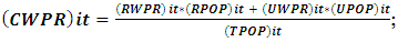Where, RWPR denotes rural work participation rate, UWPR denotes urban work participation rate, RPOP denotes rural population, UPOP denotes urban population, TPOP denotes total population, i denotes the cross-section of states and t denotes current period.

3.2. Tools for Empirical Testing

1. The study uses panel data consisting of 15 major states of India for the referred period. Firstly, all models are estimated by three popular and convenient test techniques of panel data analysis viz., the fixed-effect model (FEM), the random effect model (REM) and the pooled regression (OLS) and later only the fittest model is applied for the empirical test.

i. The random effect model is the fittest model if the probability value of the test statistic of Breusch-Pagan LM test for random effect (χ2) is statistically significant at a certain level and if the probability value of the test statistic of Hausman specification test (χ2) is statistically not significant at a certain level.

ii. The fixed effect model is the fittest if the probability value of the test statistic of Breusch-Pagan LM test for random effect (χ2) is statistically significant at a certain level, if the probability value of the test statistic of FEM (F) is statistically significant at a certain level and if the probability value of the test statistic of Hausman specification test (χ2) is statistically significant at a certain level.

iii. Ordinary least square model is the fittest model if the probability value of the test statistic of Breusch-Pagan LM test for random effect (χ2) is statistically not significant at a certain level, if the probability value of the test statistic of FEM (F) is statistically not significant at a certain level and if the probability value of the test statistic of Hausman specification test (χ2) is statistically not significant at a certain level.

As explained earlier the Gini coefficient and Lorenz curve have not satisfaction, we should consider any other family of inequality measure. In the discussion about different measures of inequality, both Sen (1973) [16] and Kolm have found that standard deviation and coefficient of variation satisfy the basic properties of absolute and relative measures of inequality respectively. Kolm has observed that these measures though satisfy the ‘income transfer principle’; they fail to satisfy the ‘principle of diminishing income transfer’. Sen rejects these measures on three grounds one of which is their failure to satisfy the ‘principle of diminishing income transfer’. The second reason is the way the deviations are taking in the formula of standard deviation and coefficient of variation. According to Sen deviations of income from the mean is less reasonable than deviations of one income from the other. The third reason lies in the squaring principle applied in the formula of standard deviation and coefficient of variation. He finds no justice in applying this principle; rather he finds that this squaring principle is making the increase in inequality from regressive transfer invariant to the levels of income of the two individuals hence dissatisfying the ‘principle of diminishing income transfer’. However, the second reason shown by Sen is not tenable because standard deviation can also be expressed as 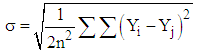. The squaring principle in standard deviation and coefficient of variation that makes them not to satisfy the ‘principle of diminishing income transfer’ can be said to be unreasonable if we are convinced of the principle of diminishing income transfer but cannot be said to be more unreasonable than the measures in the Gini family. In the Gini family, a regressive transfer of an amount between two poor persons with an income difference may lead to a less increment in inequality than a regressive transfer of the same amount between two rich persons with the same income difference if the number of persons between the two poor persons is less than that between the two rich persons. This property makes them more unreasonable than those in the SD-CV family. The ‘principle of diminishing income transfer’ is put forward on the ground of diminishing marginal utility of income. The standard deviation of the logarithm of income is tried as a solution, but has not succeeded to be reasonable for other reasons. Diminishing marginal utility of income leads to a higher welfare loss from a regressive transfer of an amount between two poor persons with an income difference than a regressive transfer of the same amount between two rich persons with the same income difference. This also leads to a larger increase in the inequality in the welfare distribution in the former case. But if we are interested in the income distribution as such and not in the implied welfare distribution then we may not bother about it. Moreover, if marginal utility diminishes at a constant rate the ‘principle of diminishing income transfer’ no longer remains reasonable, rather the inequality measures in the SD-CV family become fully reasonable.

As explained by Kolm and as is seen from the formula, SD is a per person inequality measure and thus an absolute measure of inequality. CV is a per person per rupee of mean income/expenditure inequality measure and so a relative measure of inequality. The upper bound of this relative measure is and so CV has to be divided by to have an index measure of inequality in this SD-CV family.

However, the measures of inequality in the Lorenz-Gini family are very popular in the literature though they cannot satisfy all the properties of inequality measurement. So here, we consider two families of inequality measurement – the Lorenz-Gini family on the one hand, and the SD-CV family on the other, and use three separate measures viz., a relative measure of inequality, an absolute measure of inequality, and an index measure of inequality under each family for judging the robustness of the results.

4. Findings

This section takes some of the above implications to the data. Section 4.1 describes the empirical specification for this work. Section 4.2 discusses the results.

4.1. Empirical Specification

The empirical specification is organised as follows. Let, CINEQ denotes all types of combined income/expenditure inequality (relative inequality, index of inequality and absolute inequality) in major states of India. PCELEEXP denotes per capita public expenditure on elementary education. PCSECEXP denotes per capita public expenditure on secondary education. PCHIGEXP denotes per capita public expenditure on higher education. GrNSDP denotes growth rate of net state domestic product. TPOP denotes total population. CMPCE denotes combined monthly per capita consumption expenditure. CWPR denotes combined work participation rate. The functional relationship of the specification is

CINEQ = f {PCELEEXP (-), PCSECEXP (-), PCHIGEXP (-), GrNSDP (-), TPOP (+/-), CMPCE (+), CWPR (+)}

For the sake of econometric analysis, we construct a simple linear model and use the panel data analysis to check the robustness of the results. The signs “ + ”, “ - ” in parentheses are expected signs. Thus, the model be

CINEQ _it = α + β₁ PCELEEXP _it + β₂ PCSECEXP _it + β₃ PCHIGEXP _it + β₄GrNSDP_it +β₅TPOP_it +β₆CMPCE _it + β₇CWPR _it + U_it

U_it is random error term

i = 1, 2, 3, ..., 15 (15 major states of India)

t = 1, 2, 3, ..., 7 (1983-2012)

4.2. Basic Results

4.2a. Effects of public expenditure on education at different levels on combined relative inequality in Lorenz-Gini family:

From the estimated results presented in table 1, it is observed that, for measuring combined relative inequality in the Lorenz-Gini family, the overall explanatory power (R²) of the model is 61.31%, within groups or states or inter-temporal explanatory power (R²) is 60.94% and between groups or between states or inter-state explanatory power (R²) is 62.96%.

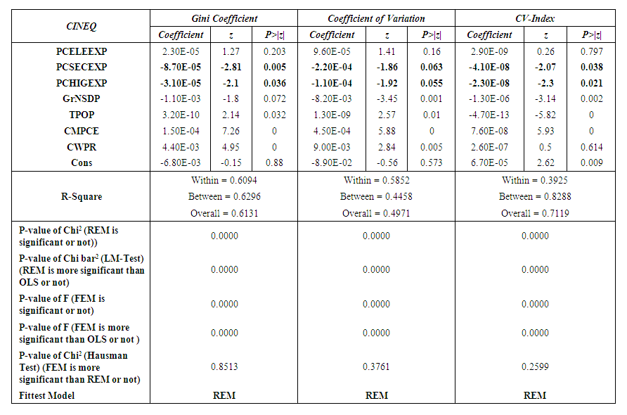Table 1. Regression result of the impact of public expenditure on education at different levels on different types of combined relative inequality and combined index of inequality in India

From table 1, it is seen that, the coefficient of per capita public expenditure on secondary education (PCSECEXP) is negative (-8.7E-05) and significant at the 1% level in explaining relative inequality in the Lorenz-Gini family in India suggesting that states with more per capita public expenditure on secondary education are associated with falling relative inequality. The relative inequality in this family will decrease by 8.7E-05 with a one rupee increase in per capita expenditure on secondary education by the governments. The coefficient of per capita public expenditure on higher education (PCHIGEXP) is negative (-3.1E-05) and significant at the 5% level in explaining relative inequality in this family in India suggesting that states with more per capita public expenditure on higher education are associated with falling relative inequality in this family. The relative inequality in this family will decrease by 3.1E-05 with a one rupee increase in per capita expenditure on higher education by the governments.

The coefficient of the growth rate of output (GrNSDP) is negative (-1.1E-03) and significant at the 10% level suggesting that states with more growth rate of output are associated with falling relative inequality in this family. The relative inequality in this family will decrease by 1.1E-03 with a one percent increase in the growth rate of output. The coefficient of the population (TPOP) is positive (3.2E-10) and significant at the 5% level suggesting that states with more population are associated with increasing relative inequality in this family. The coefficient of combined monthly per capita consumption expenditure (CMPCE) is positive (1.5E-04) and significant at the 1% level suggesting that with one rupee increase in monthly per capita consumption expenditure relative inequality in this family will rise by 1.5E-04. The coefficient of a combined work participation rate (CWPR) is positive (4.4E-03) and significant at the 1% level suggesting that a one percent increase in work participation rate relative inequality in this family will rise by 4.4E-03. However, the coefficient of per capita public expenditure on elementary education (PCELEEXP) becomes insignificant indicating that this variable has no role in explaining the relative inequality in this family.

4.2b. Effects of public expenditure on education at different levels on combined relative inequality in SD-CV family:

From the estimated results presented in table 1, it is observed that, for measuring combined relative inequality in SD-CV family, the overall explanatory power (R²) of the model is 49.71%, within groups or states or inter-temporal explanatory power (R²) is 58.52% and between groups or between states or interstate explanatory power (R²) is 44.58%.

From the table 1, it is seen that, the coefficient of per capita public expenditure on secondary education (PCSECEXP) is negative (-2.2E-04) and significant at the 10% level in explaining relative inequality in SD-CV family in India suggesting that states with more per capita public expenditure on secondary education is associated with falling relative inequality. The relative inequality in this family will decrease by 2.2E-04 with a one rupee increase in per capita expenditure on secondary education by the governments. The coefficient of per capita public expenditure on higher education (PCHIGEXP) is negative (-1.1E-04) and significant at the 10% level in explaining relative inequality in this family in India suggesting that states with more per capita public expenditure on higher education is associated with falling relative inequality in this family. The relative inequality in this family will decrease by 1.1E-04 with a one rupee increase in per capita expenditure on higher education by the governments. The coefficient of the growth rate of output (GrNSDP) is negative (-8.2E-03) and significant at the 1% level suggesting that states with more growth rate of output are associated with falling relative inequality in this family. The relative inequality in this family will decrease by 8.2E-03 with one percent increase in the growth rate of output. The coefficient of total population (TPOP) is positive (1.3E-09) and significant at the 1% level suggesting that states with more population are associated with increasing relative inequality in this family. The coefficient of combined monthly per capita consumption expenditure (CMPCE) is positive (4.5E-04) and significant at the 1% level suggesting that with a one rupee increase in monthly per capita consumption expenditure relative inequality in this family will rise by 4.5E-04. The coefficient of combined work participation rate (CWPR) is positive (9.0E-03) and significant at the 10% level suggesting that a one percent increase in work participation rate relative inequality in this family will rise by 9.0E-03. However, the coefficient of per capita public expenditure on elementary education (PCELEEXP) becomes insignificant indicating that this variable has no role in explaining the relative inequality in this family.

4.2c. Effects of public expenditure on education at different levels on combined index of inequality in SD-CV family:

From the estimated results presented in table 1, it is observed that, for measuring the combined index of inequality in SD-CV family, the overall explanatory power (R²) of the model is 71.19%, within groups or states or inter-temporal explanatory power (R²) is 39.25% and between groups or between states or interstate explanatory power (R²) is 82.88%.

From the table 1, it is seen that, the coefficient of per capita public expenditure on secondary education (PCSECEXP) is negative (-4.1E-08) and significant at the 5% level in explaining the index of inequality in SD-CV family in India suggesting that states with more per capita public expenditure on secondary education is associated with falling the index of inequality. The index of inequality in this family will decrease by 4.1E-08 with a one rupee increase in per capita expenditure on secondary education by the governments. The coefficient of per capita public expenditure on higher education (PCHIGEXP) is negative (-2.3E-08) and significant at the 5% level in explaining the index of inequality in this family in India suggesting that states with more per capita public expenditure on higher education is associated with a falling index of inequality in this family. The index of inequality in this family will decrease by 2.3E-08 with a one rupee increase in per capita expenditure on higher education by the governments. The coefficient of the growth rate of output (GrNSDP) is negative (-1.3E-06) and significant at the 1% level suggesting that states with more growth rate of output are associated with a falling index of inequality in this family. The index of inequality in this family will decrease by 1.3E-06 with a one percent increase in the growth rate of output. The coefficient of total population (TPOP) is negative (-4.7E-13) and significant at the 1% level suggesting that states with more population are associated with a decreasing index of inequality in this family. The coefficient of combined monthly per capita consumption expenditure (CMPCE) is positive (7.6E-08) and significant at the 1% level suggesting that with one rupee increase in monthly per capita consumption expenditure the index of inequality in this family will rise by 7.6E-08. However, the coefficient of per capita public expenditure on elementary education (PCELEEXP) and the coefficient of a combined work participation rate (CWPR) become insignificant indicating that these variables have no role in explaining the index of inequality in this family.

4.2d. Effects of public expenditure on education at different levels on combined absolute inequality in Lorenz-Gini family:

From the estimated results presented in table 2, it is observed that, for measuring combined absolute inequality in the Lorenz-Gini family, the overall explanatory power (R²) of the model is 90.84%, within groups or states or inter-temporal explanatory power (R²) is 95.21% and between groups or between states or inter-state explanatory power (R²) is 90.73%.

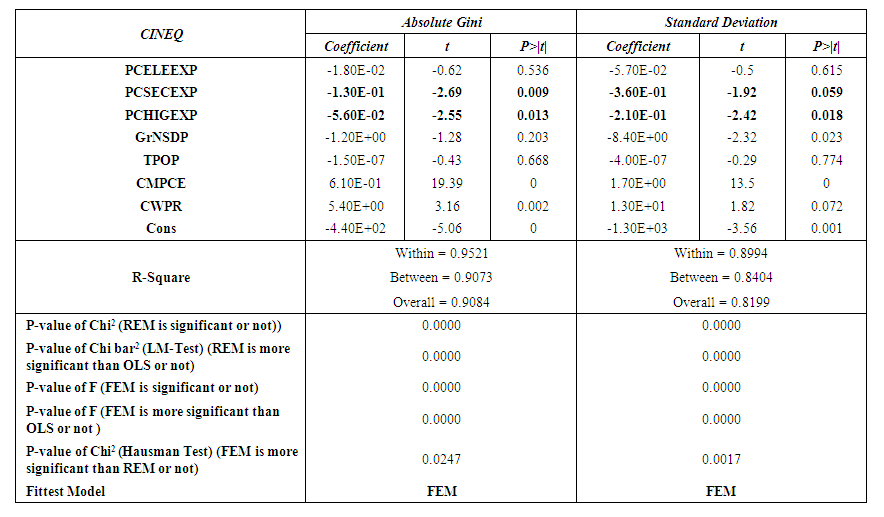Table 2. Regression result of the impact of public expenditure on education at different levels on different types of combined absolute inequality in India

From the table 2, it is seen that, the coefficient of per capita public expenditure on secondary education (PCSECEXP) is negative (-1.3E-01) and significant at the 1% level in explaining absolute inequality in the Lorenz-Gini family in India suggesting that states with more per capita public expenditure on secondary education is associated with falling absolute inequality. The absolute inequality in this family will decrease by Rs. 0.13 with one-rupee increase in per capita expenditure on secondary education by the governments. The coefficient of per capita public expenditure on secondary education (PCHIGEXP) is negative (-5.6E-02) and significant at the 5% level in explaining absolute inequality in this family in India suggesting that states with more per capita public expenditure on secondary education is associated with falling absolute inequality. The absolute inequality in this family will decrease by Rs. 0.06 with one-rupee increase in per capita expenditure on higher education by the governments. The coefficient of combined monthly per capita consumption expenditure (CMPCE) is positive (6.1E-01) and significant at the 1% level suggesting that with one rupee increase in monthly per capita consumption expenditure absolute inequality in this family will rise by Rs. 0.61. The coefficient of a combined work participation rate (CWPR) is positive (5.4E+00) and significant at the 1% level suggesting that a one percent increase in work participation rate absolute inequality in this family will rise by Rs. 5.40. However, the coefficient of per capita public expenditure on elementary education (PCELEEXP), the growth rate of output (GrNSDP) and total population (TPOP) become insignificant indicating that these variables have no role in explaining the absolute inequality in the Lorenz-Gini family.

4.2e. Effects of public expenditure on education at different levels on combined absolute inequality in SD-CV family:

From the estimated results presented in table 2, it is observed that, for measuring combined absolute inequality in SD-CV family, the overall explanatory power (R²) of the model is 81.99%, within groups or states or inter-temporal explanatory power (R²) is 89.94% and between groups or between states or inter-state explanatory power (R²) is 84.04%.

From the table 2, it is seen that, the coefficient of per capita public expenditure on secondary education (PCSECEXP) is negative (-3.6E-01) and significant at the 10% level in explaining absolute inequality in SD-CV family in India suggesting that states with more per capita public expenditure on secondary education is associated with falling absolute inequality. The absolute inequality in this family will decrease by Rs. 0.36 with a one-rupee increase in per capita expenditure on secondary education by the governments. The coefficient of per capita public expenditure on higher education (PCHIGEXP) is negative (-2.1E-01) and significant at the 5% level in explaining absolute inequality in this family in India suggesting that states with more per capita public expenditure on higher education is associated with falling absolute inequality. The absolute inequality in this family will decrease by Rs. 0.21 with a one-rupee increase in per capita expenditure on higher education by the governments. The coefficient of the growth rate of output (GrNSDP) is negative (-8.4E+00) and significant at the 5% level suggesting that states with more growth rate of output are associated with falling absolute inequality in this family. The absolute inequality in this family will decrease by Rs. 8.40 with a one percent increase in the growth rate of output. The coefficient of combined monthly per capita consumption expenditure (CMPCE) is positive (1.7E+00) and significant at the 1% level suggesting that with one rupee increase in monthly per capita consumption expenditure the absolute inequality in SD-CV family will rise by Rs. 1.70. The coefficient of combined work participation rate (CWPR) is positive (1.3E+01) and significant at the 10% level suggesting that a one percent increase in work participation rate absolute inequality in this family will rise by Rs. 13.00. However, the coefficient of per capita public expenditure on elementary education (PCELEEXP) and the coefficient of total population (TPOP) become insignificant indicating that these variables have no role in explaining the absolute inequality in this family.

5. Conclusions

The principal objective of this study is to examine what type of education expenditure is most beneficial in reducing different types of income/expenditure inequality: elementary education expenditure; secondary education expenditure; or higher education expenditure in India. From the results it appears that states that devote more resources to public secondary education and public higher education are effective in reducing all types of income/expenditure inequality in India. However, public expenditure on elementary education has no significant role in reducing any types of inequality in India. Therefore, this paper finally suggests that public expenditure on secondary education and public expenditure on higher education can be considered as very important instruments along with some other measurable factors in reducing income/expenditure inequality in India.

Notes

1. In India, both governments and private agents invest in education sector and hence total expenditure on education is divided into two categories – public expenditure on education and private expenditure on education. Variation in private expenditure for education is far greater than that of public expenditure. The opportunity cost of education for rich person is lower than that of poor person. Thus, the rich persons may able to invest a larger share of their real personal income than the poor persons do. However, per capita public education expenditure is same for all students whether they come from rich family or poor family. So we consider only public expenditure on education because for avoiding the variability in access to education and for not availability in the data of private education expenditures in India.

2. Total public education expenditure can be divided by different levels viz., expenditure on elementary education, secondary education, college & university education, technical & vocational education, training & teacher education, research etc. We divide these expenditures by three broad levels, viz., elementary education expenditure, secondary education expenditure and higher education expenditure. Expenditure on college & university education, technical & vocational education, training & teacher education, research etc. are included in higher education expenditure.

3. In India NSSO collects and publishes the raw data of consumption expenditure for rural and urban areas separately and based on these data NSSO itself calculate relative inequalities in different items for rural and urban areas separately by Gini coefficient and Lorenz curve. However, different types of overall inequalities (or better named as combined inequalities) for India and its states can be calculated by combining the rural and urban sectors together.